Single Motherhood and Headship of
Young Women
Evidence from the Census
Francine D. Blau
Lawrence M. Kahn
Jane Waldfogel
a b s t r a c t
This paper uses data from the 1970, 1980, and 1990 Censuses to investi-gate the impact of welfare benets across Metropolitan Statistical Areas (MSAs) on the incidence of single motherhood and headship for young women. A contribution of the paper is the inclusion of both MSA xed ef-fects and MSA-specic time trends to account for xed and trending un-measured factors that could inuence both welfare benet levels and fam-ily formation. In such a model, we nd no effect of welfare benets on single motherhood for whites or blacks, and a positive effect of welfare benets on single headship only for blacks.
I. Introduction
In 1996, Congress enacted legislation designed to radically overhaul the welfare system in the United States. The Personal Responsibility and Work
Op-Francine D. Blau is Frances Perkins Professor of Industrial and Labor Relations and Labor Econom-ics at Cornell University, Research Associate of the NBER, and Research Fellow of CESifo. Lawrence M. Kahn is a professor of labor economics and collective bargaining at Cornell University, and Re-search Fellow of CESifo. Jane Waldfogel is an associate professor of social work and public affairs at Columbia University. This research was supported by a grant from the Russell Sage Foundation. Debo-rah Anderson, John Cheslock, Wen-Jui Han, Elizabeth Inez Johnson, Brian Levine, Joan Moriarty, and Andre Souza provided excellent research assistance. The authors are also grateful to Al Anderson for help with the Census extracts, and to Robert Moftt and Hilary Hoynes for providing us with data on help with the Census extracts, and to Robert Moftt and Hilary Hoynes for providing us with data on welfare benets. Special thanks are due to John Bound and Harry Holzer for their considerable help in making some key data on matching Metropolitan Statistical Areas (MSAs) across Censuses available to us. The authors are also indebted to two anonymous referees for helpful comments and suggestions. The data used in this article can be obtained beginning October 2004 through September 2007 from Lawrence M. Kahn, School of Industrial and Labor Relations, Cornell University, 264 Ives Hall, Ith-aca, NY 14853– 3901.
[Submitted June 1999; accepted September 2002]
ISSN 022-166X; E-ISSN 1548-8004Ó2004 by the Board of Regents of the University of Wisconsin System
portunity Reconciliation Act of 1996 increases work requirements for welfare recipi-ents, takes away their unconditional entitlement to benets, and limits total benet receipt to ve years (Blank 1997). Part of the rationale for this legislation was a belief that Aid to Families with Dependent Children (AFDC), which up to 1996 was the major welfare program in the United States, contributed to the incidence of single-parent families. The share of children who will spend at least some portion of their childhood with a single parent now surpasses the 50 percent mark (McLana-han and Sandefur 1994). Growing up without a father present, the most common outcome in a single-parent family, is blamed for a variety of social problems, includ-ing the transmission of poverty and its consequences across generations. There is particular concern when the mother is herself very young. Although reducing single household headship (as opposed to single parenthood) was not the primary goal of the recent welfare reforms, it is also thought by some that outcomes for children are worse when single parents form their own households, rather than live with their own parents or other relatives. Again, there is particular concern when the single parent is herself very young.
An extensive literature has attempted to assess the impact of welfare on the inci-dence of single motherhood. The wide variation in benet levels across states has provided researchers with the opportunity to estimate the impact of differences in these benets on family formation outcomes.1Of course, as has been noted by many, welfare benets have been falling in real terms since the 1970s, implying that the increase in single parenthood cannot be attributed to rising welfare benets (Moftt 1998; Hoynes 1997). Nonetheless, it is still possible for decreased benet levels to lower the incidence of single motherhood, so the issue of the effect of welfare on single motherhood remains of considerable interest.
Early work on this question was based on cross-sectional analyses relating welfare benet levels in a state to the family formation decisions of women in that state (Danziger et al. 1982; Ellwood and Bane 1985; Moftt 1990). Yet, as pointed out by Ellwood and Bane (1985), Moftt (1994) and Hoynes (1997), such analyses may yield biased estimates if unmeasured factors such as state-specic norms affect both the level of welfare benets and single parenthood. For example, states where people frown upon a single-parent lifestyle may well enact low levels of welfare benets, reecting these beliefs, which may ultimately stem from religious or historical sources (for example, the culture of originally immigrating populations in a state). Or, as another example, there may be economic factors, such as labor market condi-tions, that vary systematically across states and that are not completely captured by included control variables. In both these cases, cross-sectional analyses may produce a spurious correlation between welfare benet levels and the incidence of single parenthood. This possibility has led researchers such as Moftt (1994) and Hoynes (1997) to estimate xed-effects models that in principle control for the impact of these unmeasured factors.
Yet even xed-effects methods may yield biased estimates if there are unmeasured
changesin norms or other factors that are correlated with changes in welfare benets. For example, states where the stigma placed on single parents is eroding faster may enact larger increases in welfare benet levels and experience larger increases in
single parenthood, or more rapidly deteriorating economic conditions in a state may result in larger increases in both welfare benets and single parenthood. Further examples are provided by the “tax revolt” in California in 1978 and the scal crisis in New York in 1975, which produced changes in the climate for welfare support and possibly the social acceptance of single parenthood. Merely characterizing these two states as permanently liberal (as a state xed-effect model implicitly does) misses these important changes in the scal and social climate.2
A major contribution of this paper is to address this problem by using three waves of the Census of Population (1970, 1980, and 1990) to take account not only of Metropolitan Statistical Area (MSA) xed effects, but also of changing norms and other unmeasured trending factors at the metropolitan area level, through the inclu-sion of MSA-specic time trends. An additional contribution of our paper is that the large sample sizes in the Census permit us to include more detailed measures of MSA labor and marriage market conditions than earlier research does. Our focus on MSAs is guided by the view that MSAs more closely approximate labor markets than the state-level data used in much previous work. The large sample sizes in the Census also allow us to conduct a separate analysis of less educated women. We are thus able to compare welfare effects for the less educated with average overall welfare effects, providing a sharper test of the impact of welfare than simply estimat-ing one overall welfare coefcient.
Consistent with earlier research on the impact of welfare, we nd positive cross-sectional associations between welfare benets and single motherhood and single headship. Similar to results obtained by Moftt (1994) and Hoynes (1997) who use data other than the Census, we nd that when we add MSA xed effects, some evidence of positive impacts on single headship remains for black women overall and for less educated black women, but there is no evidence of positive welfare effects for whites.3Further, adding MSA xed effects eliminates any positive welfare effect on single motherhood for all groups. Finally, when we include MSA-specic time trends, a positive effect of welfare benets on single headship for young black women overall and for young less educated black women remains, with some evi-dence of a larger effect for the less educated. We continue to nd no evievi-dence of positive welfare effects for whites (for either single motherhood or headship) or for single motherhood for blacks. We conclude that for black women, particularly the less educated, limiting welfare benets may well raise the incidence of extended family living arrangements but without affecting single parenthood. This lends sup-port to one of the most robust results obtained in this literature, initially resup-ported by Ellwood and Bane (1985) and Danziger et al. (1982), that welfare changes primar-ily affect the living arrangements of single mothers rather than single motherhood per se.
2. To some degree, changes such as those described for California and New York can be proxied by political measures such as Democratic Party representation at the state level, and in some of our analyses, we use such measures. However, changing norms and values probably inuence thebehaviorof Democrats (and Republicans), and such changes will not be captured by the standard political variables.
II. Prior Research on the Effect of Welfare on Family
Formation Outcomes and Contribution of This
Study
We are concerned with two outcomes for women: single motherhood and single mother household headship (which we call “single headship”). Each of these outcomes is joint in the sense that in order, for example, to be a single mother, one must be singleand a mother. Theories designed to explain this joint outcome must speak to both components, and in the case of single headship, the third compo-nent of heading one’s own household. Becker’s (1981) theory of marriage has pro-vided the theoretical basis for much of the empirical work on this issue. His frame-work depicts women as choosing their marriage, fertility, and household headship status to maximize their utility. Central to Becker’s (1981) theory are the opportunity cost of women’s time and the gains to specialization in marriage.
Under AFDC, welfare benets were not available to women without children (al-though programs such as disability benets or state-funded general assistance bene-ts might have been in some cases) and were unavailable or much more difcult to obtain if one was married.4 Thus, the welfare system in effect subsidized single parenthood. Further, welfare benets were more difcult to qualify for if a single parent were living with other relatives such as parents, aunts, or uncles (Ellwood and Bane 1985; Hutchens, Jakubson, and Schwartz 1989). This meant that welfare provided an especially large subsidy for single parents who headed their own house-holds. Thus, theory unambiguously predicts a positive effect of AFDC benets on single motherhood and single headship.
In addition to welfare policy, Becker’s (1981) framework predicts important roles for male and female labor market conditions in inuencing women’s choices about family formation and living arrangements. The larger the opportunity cost of a woman’s time (typically measured as better labor market opportunities), the less likely she is to choose to bear children. And the larger the gains to marriage, the more likely she is to be married. A major factor inuencing the gains to marriage is the availability of suitable partners (see, for example, Becker 1981; Wilson 1987; Ellwood and Crane 1990; Darity, Myers, and Bowman 1995). All else equal, the larger the supply of marriageable men and the better their labor market prospects, the greater women’s likelihood of being married. Moreover, the better a woman’s own labor market opportunities, the less she will gain from marriage, ceteris paribus. While better female labor markets are predicted to lower the incidence of marriage and children, their effects on the incidence of single motherhood are theoretically ambiguous. On the one hand, a better female labor market lowers the gain to marriage and thus raises the size of the group of women at risk of becoming single mothers; on the other hand, better female job prospects lower the incidence of children, reduc-ing the size of this “at risk” group. Improvements in male labor markets and greater
availability of marriageable men have similarly ambiguous theoretical effects on single motherhood. This is the case because, while they raise the likelihood that women will marry, the resulting increase in marriage (and possibly cohabitation as well) also increases the incidence of children. The higher incidence of children raises the size of the group that is at risk of eventually becoming single parents through separation, divorce, or death of a spouse. Finally, the lower the cost relative to the benets of forming one’s own household, the more likely one is to be a household head. Welfare is the primary factor considered here, although other factors such as housing costs could also play a role (Winkler 1992).5
There has been a good deal of prior empirical research on the impact of welfare on women’s family formation and fertility. In a review of this literature, Moftt (1998) reaches the following conclusions. First, studies more often than not have found that welfare benets have a negative effect on marriage and a positive effect on fertility, although often these effects are small, many studies nd no signicant effects at all, and others provide mixed results. One area in which the many studies of the impact of welfare on demographic outcomes have provided fairly consistent results is in the impact of welfare on single headship: Studies usually have found that higher welfare benets encourage single mothers to form their own households rather than to stay within households with other adult relatives (see, for example, Danziger et al. 1982; Ellwood and Bane 1985; Hutchens, Jakubson, and Schwartz 1989; Moftt 1994).6 However, even here, some negative effects also have been obtained (Moftt 1990). A second conclusion that emerges from Moftt’s (1998) review is that, when analyses are disaggregated by race, positive welfare effects tend to be larger, and are found more often for whites than for blacks, although here again there is no consistent pattern of results across the many studies that have been conducted. As we will see below, conclusions about race may be sensitive to the methodology used.
Although research on the impact of welfare benets on family formation decisions has often used cross-state variation to identify the effect of welfare, as noted above, a positive cross-sectional correlation between welfare and single headship may re-ect a state’s tolerance for single-parent households and other unmeasured factors rather than a causal effect of welfare.7This has led to the adoption in recent work by Moftt (1994) and Hoynes (1997) of a xed-effects methodology that relies on changes in welfare benet levels in a state as a potential cause of changes in single headship. In both of these studies, welfare effects on single parenthood were found to be stronger for blacks than whites. But Hoynes (1997) points out that if, in a panel data source such as the Panel Study of Income Dynamics (PSID), the composition of state populations changes over time through migration of individuals and sample attrition or entry, then the state xed-effects specication still may yield spurious
5. Unfortunately, the U.S. Department of Housing and Urban Development (HUD) has “fair-market” rent data available by MSA only since 1983. Thus, we lack the necessary information to include data on rents in our full set of analyses.
6. A recent paper by Hu (2001) points out a countervailing effect working to increase incentives for respondents younger than 18 to remain in their parent’s household when their parent is eligible for welfare: Because welfare benets increase with family size, the parent loses benets if the child (respondent) leaves the household.
results. This leads her to include individual as well as state xed effects in some of her specications.
In implementing the individual and state xed-effects design, Hoynes (1997) nds that the positive effect of welfare on single headship obtained in the state xed-effect specication disappears. This nding could mean that the positive xed-effect in models that control only for xed state effects was spurious. As Hoynes (1997) points out, the only mechanisms through which adding individual xed effects to the state xed-effects model could inuence the welfare coefcient are through mi-gration or through compositional changes over time in the PSID sample within states. Specically, if no one moved and no one left or joined the panel after the rst year, then state xed effects and individual xed effects would provide the same informa-tion.8Because only 9 percent of blacks and 16 percent of whites ever migrated in the 21 year period in Hoynes’ data, one is potentially placing a lot of weight on a relatively small number of people (the migrants, as well as sample attriters or joiners) in concluding that welfare has no effect on family formation.9
The research design pursued here uses three consecutive independent cross sec-tions from the 1970, 1980, and 1990 Censuses to examine the impact of welfare on family formation outcomes by taking into account MSA xed effects and MSA-specic time trends. As discussed above, the latter occur when norms and other trending forces are changing at different rates in different areas, while the earlier literature on welfare has assumed that these forces are xed. Since we do not have a panel of individuals, we cannot know specically whether any changes in single parenthood or in its rate of change are due to the behavior of migrants or current residents. However, by examining the characteristics of migrants, we can make some inferences about what may be driving the changes in single parenthood and headship. In an earlier paper, Blau, Kahn, and Waldfogel (2000), we examined the determi-nants of marriage. We found that in xed effects (rst difference) models estimated over the 1980– 90 period, welfare had signicantly negative effects on marriage for less educated young black and white women. These effects were larger in magnitude for blacks, similar to the xed-effects results for single headship in Hoynes (1997), and as mentioned earlier, some of the ndings in Moftt (1994). However, when we took account of heterogeneity in time trends by using second differences, the effects of welfare became small in magnitude and statistically insignicant, sug-gesting a correlation between trends in norms and other trending forces and trends in welfare benets.10
In order to estimate the effects of welfare on single parenthood and headship, we need to take into account labor and marriage market conditions, including the supply of marriageable men. Several previous studies have found that men’s employment opportunities have a positive effect on marriage for both blacks and whites.11 How-ever, the same considerations that led some researchers to use xed-effects models
8. In the models that control for state and individual xed effects, the state xed effects could reect the possibility that individuals’ tastes come to resemble those in the state where they live.
9. We return to the issue of welfare and migration later in this article.
10. Papers by Ribar and Wilhelm (1999) and Page, Spetz, and Millar (2000) on welfare caseloads also nd that it is important to control for time trends.
in estimating the effects of welfare apply here. For example, married men outearn single men (Korenman and Neumark 1991), suggesting that the high marriage rates one observes in areas with good male job opportunities may merely reect married men’s greater productivity. And our reasoning about time trends applies here as well: Improvements in married men’s job opportunities may reect secular changes in married men’s wage premium. Again, models with area-specic time trends (in addi-tion to xed effects) can in principle take account of such effects.
A common shortcoming of the literature on family formation is that studies have tended to use a fairly limited measure of labor market conditions (typically, the unemployment rate and/or average earnings). Moreover, previous studies have tended to measure labor market conditions for all men or women rather than by education and race groups separately. Much of this earlier work uses actual female and male wage or employment rates as explanatory variables, even though these will be affected by marriage and fertility decisions. Further, measures of the supply of marriageable men generally combine the effects of partner availability and labor market conditions into one measure. This study differs from previous research in using a richer and plausibly more exogenous set of measures of labor and marriage market conditions, and in using measures that are disaggregated by education and race groups. These measures are described in detail below.
A nal distinctive feature of our research design is to focus on young women— those aged 16–24. This means that we are measuring labor market conditions at roughly the time when these women are making their family formation decisions. Including older age groups, as much of the existing work does, brings in groups who made their family formation decisions at widely varying times, hence possibly under widely differing labor and marriage market conditions. Our focus on young women also means that we are concentrating on the age group that has been at the center of much of the policy concern. Of course it must be acknowledged that our results may not be representative of the behavior of women outside our age group.
III. Analytical Framework, Data, and Methodology
This study exploits MSA-level differences in welfare policy and la-bor and marriage market conditions to estimate the impact of these factors on young women’s propensity to become single parents or single heads. The analytical frame-work is based on the assumption that substitution in the labor market between groups such as high school dropouts or college graduates is imperfect. Thus, changes in relative supply of or demand for such groups will in general produce changes in relative wage offers (Katz and Murphy 1992). These in turn are expected to affect family formation decisions. As discussed above, labor and marriage market condi-tions are expected to have theoretically ambiguous effects on the incidence of single motherhood and single headship, due to opposing effects on being single and having children.
markets. In formulating this framework, our maintained hypothesis is that supply and demand adjustments across regions are partially limited by mobility costs. A considerable body of research supports this view, nding that demand or supply shifts have wage or employment-to-population ratio effects that last up to 10–15 years (Bartik 1993, 1994; Topel 1986, 1994; Bound and Holzer 1993 and 2000; Borjas and Ramey 1995).12
To analyze family formation outcomes, we use microdata on women age 16–24 from the 5 percent samples of the 1980 and 1990 Censuses and the 2 percent sample of the 1970 Census. These are the largest available samples in each year. Although macroeconomic conditions were fairly similar in the latter two years, 1970 was a mild recession year. We exploit area differences in economic activity as important explanatory variables, providing some control for economic conditions. The Census les contain sufcient observations to stratify analyses by race-education group and to identify local labor market effects within each of these categories. Our local labor markets are MSAs. Where boundaries for MSAs change over time, we use a consis-tent set of denitions so that comparable areas are dened for 1970, 1980, and 1990.13 Due to sample size considerations, we use 67 comparable MSAs that have at least ten young women in each race-education subgroup across which our supply and demand indexes are dened (see below).
In this paper, we use all blacks and all whites regardless of Hispanic ethnicity status. This decision was necessitated by the fact that Hispanics were not separately identied in the 1970 Census. For the purposes of creating labor and marriage market variables (see below), we also divide our samples of young women into three educa-tion groups: Those with less than a high school educaeduca-tion; those who have completed high school but have no further education; and those who have completed some college beyond high school (this latter category includes both those with some col-lege and those with a colcol-lege degree). In some analyses, we estimate separate equa-tions for the less educated group because we expect welfare to have larger effects for them than for the whole population.
A single mother is dened as a woman who is not currently married and who is coded by the Census as the mother of children under 18 living in the household.14
12. However, Blanchard and Katz (1992) argue that migration undoes regional demand effects within a decade.
13. Because of changing denitions, these MSAs were created by matching as closely as possible the metropolitan areas as dened by the Census. We were guided by Bound and Holzer’s (2000) original breakdown of these areas. In some cases, MSAs were consolidated so that we only know the probability that an individual is in a particular MSA. When this relatively rare event occurred, we included individuals only if they had a greater than 0.5 probability of living in a particular MSA, and we assigned them to this MSA. In an Appendix available upon request, we provide further details as well as a list of the included MSAs.
A single head is dened as a single mother who is also head of the household. The analysis uses microdata on individuals to estimate the impact of welfare benets on family formation. The following probit model for the determinants of single mother-hood (headship) for personi,in metropolitan areajand yeartis estimated separately by race:
(1) P(Yijt51)5F(Vijtbt1Cjtw),
whereYis a dummy variable signifying that one is a single mother (head),F(-) is the standard normal cumulative distribution function, Vis a vector of individual characteristics,C is a vector of MSA-specic factors, andbandw are coefcient vectors.
In the vector V, we control for measured characteristics available in the census data which would be expected to affect an individual’s labor market prospects, their attractiveness as a marriage partner, and their preferences regarding marriage and motherhood. Thus, although our age group is relatively narrow, we take advantage of the large sample sizes available in the Census to include individual age dummy variables in years, as well as schooling dummy variables referring to different levels of schooling. Specically, we include controls for the following educational catego-ries: 0 years completed, 1–4 years, 5–8 years, 9 years, 10 years, 11 years, 13–15 years, and 16 years and older. The omitted category is those with exactly 12 years completed.15
We include those enrolled as well as those not enrolled in school because school-ing decisions are made in the same context as marriage and childbearschool-ing decisions. Thus, in effect we estimate reduced form models for single parenthood and headship. While we acknowledge that the education variable may be endogenous, we also believe that it is especially important to control for this in analyzing the impact of welfare, as has virtually every study of the impact of welfare. Since our samples are young and include the enrolled, the within-group control for age is important: the meaning of having less than a high school education, for instance, is not the same for someone age 16 (who may be continuing on) as it is for someone age 22 (who has likely completed her education). Our inclusion of individual age dummy variables controls for cross-MSA differences in the age composition of the popula-tion and thus allows for an appropriate interpretapopula-tion of the coefcients on the MSA-level variables (C).
In the vector C, we include a measure of welfare generosity which is of course the key explanatory variable of interest. Welfare benet levels are measured as the log of the sum of 0.7 times the maximum AFDC benet plus food stamp benets available for a family of four in the state in which the MSA is located in 1980 dollars.16We also include the following MSA-level control variables: The adult male
a recent analysis of the effects of welfare on cohabitation decisions, see Moftt, Reville, and Winkler (1998).
15. In calculating years of education, we follow Jaeger (1997) to deal with the changes that were made to the education questions beginning in the 1990 Census.
(ages 25–54) unemployment rate and the log of the adult male average wage level in the labor market as measures of overall indicators of labor market conditions. Further, controlling for wage levels puts a sharper interpretation on the welfare bene-t variable, since average hourly wages are likely to be closely correlated with local living costs. In addition, adult wages and unemployment are less likely to be endoge-nous to the behavior of the younger age group employed in our primary analyses than measures that include younger individuals. Wages were expressed in 1980 dol-lars and computed as the previous year’s annual earnings divided by the product of weeks worked and average weekly work hours among the non self-employed.17
Finally in each model, we include indexes (dened below) of labor market demand and supply for young men and young women in each of 12 race-gender-education groups of 16–24 year olds: (white, black) x (male, female) x (ED,12,ED512,
ED.12). Because we use estimates of the underlying supply and demand conditions that determine wage and employment opportunities, rather than the actual earnings and employment of the young women and their potential partners as explanatory variables, our approach is less likely to be contaminated by reverse causality biases than much previous work. Each equation has 12 supply variables and 12 demand variables, and the model thus allows supply and demand for a given group (for example, black men with 12 years of schooling) to inuence the family formation decisions of each of the race-education groups of women studied here. Taken to-gether, the demand and supply indexes control for the underlying determinants of each group’s labor market prospects as well as the pure supply of potential partners. We followed the approach of including the full set of supply and demand variables for each observation because it did not in any way constrain the coefcients on the supply and demand variables or require us to make any a priori assumptions about likely marriage patterns.18
A group’s supply and demand indexes are dened as:
(2) Supplykjt5ln (Skjt)
(3) Demandkjt5ln (Dkjt),
living arrangements. The authors used a telephone survey of state agencies to collect data on this difference at one point in time (the mid-1980s). However, such data are not available on the time series basis necessary to use in our analyses. We note, however, that Hutchens, Jakubson, and Schwartz nd for all states that it was easier to qualify for benets as a household head than as a single mother in an extended family. Thus, our welfare benet variable should at least be positively correlated with the gains to being a single mother household head.
17. Those with computed hourly wages less than $1 or greater than $250 in 1980 dollars were excluded from the calculations.
where k stands for gender-education-race group of 16–24 year olds, jfor MSA, t for year, Skjt is the fraction of the MSA’s total population comprised by group k,
andDkjtis a demand index in yeartfor group k. The demand indexes are similar to
those constructed by Katz and Murphy (1992) and are dened as follows:
(4) Dkjt 5 So(sokt*Eojt/Ejt),
whereoindexes industry-occupation category (14 industries crossed with three oc-cupations),19 s
oktis the share that group k comprises of total U.S. employment in
industry-occupation cell o; andEojtandEjt are respectively MSAjemployment in
industry-occupation celloand total MSAjemployment.
The demand index is essentially a predicted MSA employment share for groupk
in MSA j,where we weight the relative employment of industry-occupation group
o in areajby the national importance of group k in the industry-occupation cell. Since the same weights (sok) are used for each MSA in a given year, the demand
index is driven by area differences in overall industry-occupation composition of employment. The supply index is the group’s actual population share that is thus in similar units as the predicted employment share in the demand index.
Of course, these demand and supply indexes may be affected by relative wages and are therefore not precisely the same as the desired notion of the placement of the local relative demand and supply curves (Katz and Murphy 1992). However, because the demand index is based on national employment shares for the group in each industry-occupation cell and overall local employment in each industry-occupation cell, it is not likely to be greatly affected by changes in our focal groups’ local wage levels. Furthermore, the supply index refers topopulation
rather than employment shares, again providing perhaps a more convincing source of exogenous variation, although even the population of a given race-gender-education group may be affected by relative wages through migration and schooling decisions.20
Equation 1 is estimated on a pooled 1970– 1980– 1990 sample with MSA dummy variables, MSA-specic time trends,21and overall time effects. We compute Huber-White standard errors and allow for correlation of the errors within each MSA.22In each of the models, we allow the coefcients of the individual-specic variables to be different in different time periods by interacting them with the year dummy variable(s).
19. The industry categories are: Agriculture, Forestry and Fisheries; Mining; Construction; Manufacturing (Durable Goods); Manufacturing (Nondurable Goods); Transportation, Communications, and Other Public Utilities; Wholesale Trade; Retail Trade; Finance, Insurance, and Real Estate; Business and Repair Ser-vices; Personal Services Including Private Households; Entertainment and Recreation SerSer-vices; Profes-sional and Related Services; and Public Administration. The three occupation groups are: ProfesProfes-sional, Technical and Managerial; Clerical and Sales; Craft, Operative, Laborer and Service.
20. The demand index as dened above uses employment shares and the current year national employment share weights. Our results were the same when we used shares of work hours instead of employment. 21. The MSA-specic time trends are equal to the MSA dummy variables multiplied by YEAR, where YEAR51970, 1980, 1990.
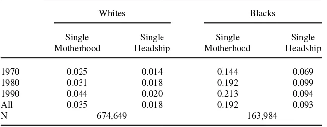
Table 1
Mean Values for the Regression Sample
Whites Blacks
Single Single Single Single
Motherhood Headship Motherhood Headship
1970 0.025 0.014 0.144 0.069
1980 0.031 0.018 0.192 0.099
1990 0.044 0.020 0.213 0.094
All 0.035 0.018 0.192 0.093
N 674,649 163,984
Notes: A single mother is dened as a woman who is not currently married and who is the mother of a child or children younger than 18 living in the household. A single head is dened as a single mother who is also head of the household.
IV. Results
A. Sample Means
Table 1 shows sample means of the dependent variables for the underlying 1970, 1980, and 1990 Census microdata for the 67 MSAs upon which our regression analy-sis is based. While our 67 MSAs constitute only a subset of the population, national means are virtually identical to those reported in Table 1.23The data in Table 1 reect some well-known national patterns. In each year, black women are considerably more likely to be single mothers and single heads than are white women. The data also show an increase in the incidence of single motherhood and single headship for both blacks and whites over the 1970– 90 period taken as a whole, although, especially for blacks, there was some leveling off in the trends over the 1980s.
At the aggregate level, it is difcult to attribute the observed increases in single motherhood to welfare benets, since benets declined by an average of about 18 percent in real terms in our MSA sample between 1970 and 1980, and fell by 9 percent between 1980 and 1990. Thus not only have welfare benets been falling during this period of rising single motherhood; they fell faster during the period when this outcome was increasing fastest for black women. It is still possible, however, for welfare benets to be a determinant of single motherhood, and our regression analy-ses attempt to estimate this effect.
B. Basic Probit Regression Results
The probit results for the welfare benet variable are presented in Tables 2 (white women) and 3 (black women). The entries are the partial derivative of the dependent variable with respect to the welfare benet measure evaluated at the mean of the dependent variable. The tables present results for cross-sectional models (Panel A), models with MSA dummies (Panel B), and models with MSA dummies and MSA-specic trends (Panel C). For purposes of comparison, within each panel, we present models for all women and for those with less than 12 years of schooling. We also report results for two specications: models with the adult male log wage and unem-ployment rate included, and models with these two indicators plus our 24 supply and demand variables.
Despite the large number of specications, some general patterns emerge. First, in the cross-sectional models (Panel A of Tables 2 and 3), welfare has positive coef-cients for both single motherhood and single headship for whites and blacks. More-over, these effects are signicant in each case for whites and for single headship for blacks. The estimated derivatives tend to be larger for the less educated than for the full sample, although the differences are not large among blacks. Thus, the results indicate that without taking into account MSA xed effects or trends, it appears that welfare encourages single motherhood for whites and single headship for both whites and blacks.
When we add MSA xed effects (Tables 2 and 3, Panel B), the positive effects for whites all become negative, with several of them statistically signicant. The single motherhood results for blacks remain insignicant and usually positive, while the black single headship results remain positive, with two of them marginally signicant—all education groups pooled with the full set of labor market variables, and the less educated with just adult male wages and unemployment included. These results are qualitatively similar to previous ndings using state xed effects that found a welfare effect on single headship only among blacks (Moftt 1994 in one specication; Hoynes 1997).
Finally, we turn to the results that take into account both MSA xed effects and MSA-specic trends (Tables 2 and 3, Panel C). These specications continue to show no evidence of positive welfare effects for whites. In the second model shown (that is, with the full set of labor market variables), the effects of welfare for whites are insignicant three times and signicantly negative once (single motherhood, edu-cation , 12). As mentioned earlier, Moftt (1990) has pointed out that in some studies welfare has been found to have negative effects on single headship, a seem-ingly counterintuitive nding. In any event, for whites at least, carefully controlling for omitted variables by including MSA dummies and trends eliminates the apparently positive effects of welfare found in the cross-sectional results (Table 2, Panel A).
B
la
u
,
Ka
hn,
and
Wa
ldfoge
l
395
parentheses)
All Education Groups Pooled Education,12 Only
Specication Single Mother Single Head Single Mother Single Head
A. Cross-section
Adult male log wages and 0.0083 ** 0.0124 ** 0.0184 ** 0.0236 **
unemployment included (0.0037) (0.0049) (0.0083) (0.0117)
Adult male log wages and
unemployment and all group supply 0.0100 *** 0.0114 *** 0.0185 *** 0.0214 ***
and demand indexes included (0.0031) (0.0027) (0.0046) (0.0038)
B. MSA dummies
Adult male log wages and 20.0171 ** 20.0107 20.0227 ** 20.0235
unemployment included (0.0086) (0.0088) (0.0115) (0.0159)
Adult male log wages and
unemployment and all group supply 20.0094 20.0045 20.0200 * 20.0078
and demand indexes included (0.0067) (0.0057) (0.0104) (0.0097)
C. MSA dummies and MSA trends
Adult male log wages and 20.0166 ** 20.0053 20.0345 *** 20.0094
unemployment included (0.0080) (0.0056) (0.0098) (0.0098)
Adult male log wages and
unemployment and all group supply 20.0115 0.0047 20.0602 *** 20.0144
and demand indexes included (0.0105) (0.0083) (0.0214) (0.0165)
Notes: A single mother is dened as a woman who is not currently married and who is coded by the Census as the mother of children younger than 18 living in the household. A single head is dened as a single mother who is also head of the household. Coefcients are from probit models. Standard errors are heteroskedasticity-robust and are corrected for correlation within MSAs. Control variables include age and education dummies, whose effects are allowed to vary by year. Sample sizes are: Pooled5674,649; ED,125227,144.
The
Journa
l
of
Hum
an
R
es
ource
s
Table 3
Derivatives for the Effect of Welfare Benets Evaluated at Dependent Variable Mean: Blacks (asymptotic standard errors in parentheses)
All Education Groups Pooled Education,12 Only
Specication Single Mother Single Head Single Mother Single Head
A. Cross-section
Adult male log wages and 0.0189 0.0708 *** 0.0236 0.0827 ***
unemployment included (0.0258) (0.0216) (0.0307) (0.0259)
Adult male log wages and
unemployment and all group supply 0.0200 0.0487 *** 0.0235 0.0430 *
and demand indexes included (0.0193) (0.0175) (0.0273) (0.0221)
B. MSA Dummies
Adult male log wages and 0.0007 0.0519 0.0491 0.0800 *
unemployment included (0.0462) (0.0498) (0.0463) (0.0480)
Adult male log wages and
unemployment and all group supply 20.0037 0.0483 0.0100 0.0309
and demand indexes included (0.0360) (0.0295) (0.0476) (0.0393)
C. MSA dummies and MSA trends
Adult male log wages and 20.0050 0.0265 0.0149 0.0759
unemployment included (0.0588) (0.0439) (0.0584) (0.0570)
Adult male log wages and
unemployment and all group supply 20.0179 0.0812 * 0.0043 0.1194 **
and demand indexes included (0.0549) (0.0443) (0.0741) (0.0567)
Notes See notes to Table 2 for further explanation. Sample sizes are: Pooled5163,984; ED,12567,952.
standard error 0.057) for less educated black women. At the mean frequency of single headship for each group, these derivatives correspond to elasticities of 0.871 for the full sample and 1.312 for those with education less than 12 years. This pattern of elasticities is consistent with our expectation that welfare would have larger effects for those with lower potential market wages, as is the fact that welfare has more a positive effect on black than white women (due to black women’s lower income levels). In sum, for black women in general and especially for less educated blacks, these results imply that while welfare raises the likelihood that single mothers will form their own households, it does not raise the incidence of single motherhood itself. As noted above, this is one of the most robust results in the prior literature on the effects of welfare on demographic outcomes. The larger size and signicance of the coefcients when the group-specic supply and demand variables are included suggests the importance of taking into account group-specic indicators of labor market conditions, rather than simply aggregate indicators.
Although we have found some evidence that, for young black women, welfare benets are positively associated with single headship, the census data do not allow us to determine whether this effect is due to the family formation decisions of women who live in a particular area or the attraction of single heads to high benet areas. This ambiguity characterizes all research that uses single cross-sections or pooled cross sections such as multiple years of the Census or the Current Population Survey, and is present to some extent even in Hoynes’ (1997) panel data model including both individual and state effects. In the latter case, while we do know whether the dependent variable, single headship, has changed for the individual, a positive effect of welfare benets on single headship could still reect either a change in headship in response to welfare benet levels after an exogenous move or a prior decision to become a single head and hence move to a high benet state. Thus, short of a multi-equation model of migration and family formation, which would be extremely hard to credibly identify, we cannot, even with panel data, denitively resolve the migra-tion issue.
C. Supplementary Results
While our focus in this paper is the impact of welfare on family formation decisions, it is also of some interest to consider the impact of the personal characteristics and labor market variables. Selected results for these variables for the incidence of single headship are shown in Table 4 for the specication that includes MSA dummies and MSA trends. The age and education results reported in the Table are the estimated main effects of these variables. They measure the impact of these variables for 1970, since the equations also include age and education interactions with 1980 and 1990 dummy variables. The main effects indicate that, as would be expected, the incidence of single headship rises with age (the omitted category is age 24) and falls with education level (the omitted category is ed 12), all else equal. Our ndings for the interactions of these variables with the year dummies, which are not shown in the Table, indicate that the incidence of single headship in 1980 and 1990 fell relative to 1970 for the very young (ages 16 and 17) and for those with some college educa-tion. These latter ndings for education are consistent with results reported by Blau (1998), who found that the relationship between single parenthood and education became more negative over this period.
The coefcients for the 24 group-specic supply and demand variables are highly signicant as a group. When these variables are excluded, the overall labor market indicators (adult male log wages and unemployment) are jointly signicant and indi-cate that higher overall wages and lower overall unemployment are negatively asso-ciated with single headship for whites and blacks. However, when we add the supply and demand variables, the overall wage and unemployment effects become insig-nicant individually and jointly. Perhaps the group-specic supply and demand vari-ables capture labor and marriage market conditions more accurately than the overall labor market indicators (wage and unemployment levels) that most previous research has employed.
D. Alternative Specications
In addition to the specications shown in Tables 2 and 3, we found that the basic results for welfare benets were robust to a variety of alternative specications. First, in addition to the regular AFDC and food stamps programs, in 1980 25 states plus Washington, D.C. offered AFDC in some cases to married-couple families through the AFDC-Unemployed Parent (AFDC-UP) program.24The Family Support Act of 1988 required all states to offer AFDC-UP by October 1990, and they all did. But we do not know whether they began offering it by the spring of 1990 when the Cen-sus interviews were conducted. Despite this ambiguity in the timing of AFDC-UP coverage, we estimated supplementary models with a dummy variable for AFDC-UP coverage as of 1970, 1980, or 1988 for the corresponding regressions. The ndings for welfare benet levels are very similar to those without controlling for AFDC-UP coverage.
Second, our models with MSA xed effects and MSA-specic trends are an at-tempt to account for otherwise unmeasured variables and their trends that could
B
la
u
,
Ka
hn,
and
Wa
ldfoge
l
399
Dependent Variable-Single Head
Explanatory Variables Whites Blacks
Age 16 20.0875*** 20.0875*** 20.4090*** 20.4093***
(0.0036) (0.0036) (0.0241) (0.0241)
Age 17 20.0705*** 20.0705*** 20.3299*** 20.3308***
(0.0032) (0.0031) (0.0168) (0.0169)
Age 18 20.0473*** 20.0473*** 20.2209*** 20.2207***
(0.0030) (0.0030) (0.0122) (0.0123)
Age 19 20.0319*** 20.0319*** 20.1632*** 20.1625***
(0.0022) (0.0022) (0.0080) (0.0080)
Age 20 20.0212*** 20.0212*** 20.0976*** 20.0973***
(0.0014) (0.0014) (0.0103) (0.0103)
Age 21 20.0159*** 20.0158*** 20.0599*** 20.0598***
(0.0019) (0.0019) (0.0068) (0.0067)
Age 22 20.0085*** 20.0085*** 20.0351*** 20.0351***
(0.0014) (0.0015) (0.0073) (0.0072)
Age 23 20.0056*** 20.0056*** 20.0339*** 20.0338***
(0.0012) (0.0012) (0.0073) (0.0073)
Ed0 0.0259*** 0.0259*** 0.0806*** 0.0807***
(0.0044) (0.0044) (0.0209) (0.0205)
Ed1 to 4 0.0221*** 0.0220*** 0.0563* 0.0589*
The
Journa
l
of
Hum
an
R
es
ource
s
Table 4(continued)
Dependent Variable-Single Head
Explanatory Variables Whites Blacks
Ed5 to 8 0.0240*** 0.0240*** 0.1043*** 0.1054***
(0.0053) (0.0053) (0.0086) (0.0086)
Ed9 0.0292*** 0.0292*** 0.1074*** 0.1075***
(0.0023) (0.0023) (0.0086) (0.0085)
Ed10 0.0238*** 0.0238*** 0.0938*** 0.0945***
(0.0021) (0.0020) (0.0067) (0.0067)
Ed11 0.0149*** 0.0148*** 0.0617*** 0.0617***
(0.0016) (0.0016) (0.0101) (0.0101)
Ed13 to 15 20.0129*** 20.0129*** 20.0673*** -0.0681***
(0.0013) (0.0013) (0.0083) (0.0084)
Ed16 and over 20.0263*** 20.0262*** 20.1412*** 20.1410***
(0.0027) (0.0027) (0.0326) (0.0327)
Log adult male wage 20.0254*** 20.0141 20.1973*** 0.0640
(0.0076) (0.0137) (0.0614) (0.0981)
Adult male unemployment rate 0.0557 0.0125 0.2315 0.0823
(0.0344) (0.0454) (0.1842) (0.3683)
Supply and demand variables? no yes no yes
Joint tests
Adult male wages and unemployment p50.0016 p50.5818 p50.0019 p 50.7456
Supply and demand variables — p,.0000 — p,.0000
Notes: Entries are partial derivatives evaluated at dependent variable means. Other control variables include: year dummy variables, age and education interactions with year dummies, MSA dummies, and MSA trends. The age and education coefcients are main effects that measure the impact of these variables for 1970, since the equations also include age and education interactions with 1980 and 1990 dummy variables. Reference categories are 12 years for education and 24 years old for age. *** Signicantly different from zero at the 1 percent level on a two-tailed test.
affect both welfare benets and family formation decisions. Yet even controlling for such trends may not adequately account for unmeasured variables that could bias even the second difference equations. We attempted to control for such factors by adding to some specications variables reecting the political climate in each state. Specically, we include: the fraction of the state’s lower house comprised of Demo-cratic party members; the fraction of the upper house that was DemoDemo-cratic; and an indicator variable for whether the governor was Democratic.25When these variables were added, the results for the welfare benet variable were virtually identical to those reported in Tables 2 and 3, giving us further condence that we have adequately controlled for omitted variables.
V. Conclusions
This paper has used data from the 1970, 1980, and 1990 Censuses to investigate the impact of welfare benets on the incidence of single parenthood and headship for young women. We controlled for personal characteristics, labor, and marriage market conditions, and unlike most previous research on the impact of welfare, metropolitan area xed effects and MSA-specic time trends. The impor-tance of controlling for MSA xed effects and trends is that area-specic factors such as norms or other unmeasured economic or social factors and their trends may affect both the provision of welfare benets and individual family formation deci-sions. The large sample size of the Census also allows us to control for labor and marriage market conditions in a more detailed way than in previous work. Stratifying by race, we estimated the impact of welfare benets on single motherhood and single headship for individuals overall and separately for the less educated, a group we expect to be disproportionately affected by welfare.
Consistent with earlier research on the impact of welfare, we nd positive cross-sectional associations between welfare benets and single parenthood and headship. However, these cross-sectional associations may reect unmeasured factors such as norms that inuence single parenthood or headship and welfare benets levels. Simi-lar to results obtained in recent studies by Moftt (1994) and Hoynes (1997), using data other than the Census, we nd some evidence that the positive effects on single headship remain for black women but largely disappear for whites when MSA xed effects are included. However, even a specication including such MSA xed effects does not account for unmeasured factors such as changing norms and other trending forces that cause changing levels of both welfare benets and single headship. The use of three waves of Census data enables us to account for these factors by including MSA-specic time trends. In these analyses, a positive effect of welfare benets on single headship for young black women and an even larger positive effect for young less-educated black women remains. We conclude that for young black women, cur-tailing welfare benets may well raise the likelihood that single mothers live in extended family arrangements but without affecting the likelihood that they become
single mothers in the rst place. This might be expected to benet children who may be more likely to live with multiple adult relatives than otherwise, but much depends on the circumstances of the individual family (Moore and Brooks-Gunn, 2002). Regardless of its effect on child well-being, a reduction in single headship, rather than single motherhood itself, is clearly not the main outcome that welfare reformers had in mind when they enacted the federal reforms of 1996, and the state reforms that preceded them. Our results regarding single parenthood conrm those of much of the earlier literature: welfare benets seem not to be an important motiva-tor for young women to have children out of wedlock.
References
Bartik, Timothy J. 1993. “Who Benets from Local Job Growth: Migrants or the Original Residents?” Regional Studies 27(4):297– 311.
———. 1994. “The Effects of Metropolitan Job Growth on the Size Distribution of Family Income.”Journal of Regional Science34(4):483– 501.
Becker, Gary S. 1981.A Treatise on the Family.Cambridge, Mass.: Harvard University Press.
Blanchard, Olivier, and Lawrence F. Katz. 1992. “Regional Evolutions.” Brookings Papers on Economic Activity1:1–61.
Blank, Rebecca M. 1997. “Policy Watch: The 1996 Welfare Reform.”Journal of Eco-nomic Perspectives 11(3):169– 77
Blau, Francine D. 1998. “Trends in the Economic Well-Being of Women: 1970-1995.”
Journal of Economic Literature 36(1):112– 65.
Blau, Francine D., Lawrence M. Kahn, and Jane Waldfogel. 2000. “Young Women’s Mar-riage Rates in the 1980s: The Role of Labor and MarMar-riage Market Conditions.” Indus-trial and Labor Relations Review53(4):624– 47.
Borjas, George J., and Valerie Ramey. 1995. “Foreign Competition, Market Power, and Wage Inequality.” Quarterly Journal of Economics110(4):1075– 1110.
Bound, John, and Harry Holzer. 1993. “Industrial Shifts, Skills Levels, and the Labor Mar-ket for White and Black Males.”Review of Economics and Statistics 75(3):387– 96.
Bound, John, and Harry Holzer. 2000. “Demand Shifts, Population Adjustments, and Labor Market Outcomes during the 1980s.”Journal of Labor Economics 18(1):20– 54.
Brien, Michael J. 1997. “Racial Differences in Marriage and the Role of Marriage Mar-kets.”Journal of Human Resources32(4):741– 78.
Danziger, Sheldon, George Jakubson, Saul Schwartz, and Eugene Smolensky 1982. “Work and Welfare as Determinants of Female Poverty and Female Headship.”Quarterly Jour-nal of Economics97(3):519– 34.
Darity, William A., Jr., Samuel L. Myers, and Phillip Bowman. 1995. “Family Structure and the Marginalization of Black Men: Policy Implications.” InThe Decline in Mar-riage Among African-Americans: Causes, Consequences and Policy Implications, ed. M. Belinda Tucker and Claudia Mitchell-Kernan, 263– 308. New York, N.Y.: Russell Sage Foundation.
Ellwood, David, and Mary Jo Bane. 1985. “The Impact of AFDC on Family Structure and Living Arrangements.” Research in Labor Economics7:137– 207.
Ellwood, David, and Jonathan Crane. 1990. “Family Change among Black Americans: What Do We Know?”Journal of Economic Perspectives 4(4):65– 84.
Hoynes, Hilary Williamson 1997. “Does Welfare Play Any Role in Female Headship Deci-sions?”Journal of Public Economics 65(2):89– 117.
Hutchens, Robert M., George Jakubson, and Saul Schwartz. 1989. “AFDC and the Forma-tion of Subfamilies.”Journal of Human Resources 24(4):599– 628.
Hu, Wei-Yin. 2001. “Welfare and Family Stability: Do Benets Affect When Children Leave the Nest?”Journal of Human Resources 36(2):274– 303.
Jaeger, David. 1997. “Reconciling the Old and New Census Bureau Education Questions: Recommendations for Researchers.” Journal of Business and Economic Statistics 15(3): 300–309.
Katz, Lawrence F., and Kevin M. Murphy. 1992. “Changes in Relative Wages, 1963– 1987: Supply and Demand Factors.”Quarterly Journal of Economics107(1):35– 78.
Korenman, Sanders, and David Neumark. 1991. “Does Marriage Really Make Men More Productive?” Journal of Human Resources26(2):282– 307.
Lichter, Daniel T., Felicia B. LeClere, and Diane K. McLaughlin. 1991. “Local Marriage Markets and the Marital Behavior of Black and White Women.”American Journal of So-ciology96(4):843– 67.
London, Rebecca. 1998. “Trends in Single Mothers’ Living Arrangements from 1970 to 1995: Correcting the Current Population Survey.”Demography, 35(1):125– 31.
Mare, Robert D., and Christopher Winship. 1991. “Socioeconomic Change and the Decline of Marriage for Blacks and Whites.” InThe Urban Underclass,ed. Christopher Jencks and Paul E. Peterson, 175–202. Washington, D.C.: Brookings Institution.
McLanahan, Sara, and Gary Sandefur. 1994.Growing Up with a Single Parent: What Hurts, What Helps?Cambridge, Mass: Harvard University Press.
Moftt, Robert. 1990. “The Effect of the U.S. Welfare System on Marital Status.”Journal of Public Economics41(1):101– 24.
———. 1992. “Incentive Effects of the U.S. Welfare System: A Review.”Journal of Eco-nomic Literature30(1):1– 61.
———. 1994. “Welfare Effects on Female Headship.”Journal of Human Resources29(2): 621–36.
———. 1998. “The Effect of Welfare on Marriage and Fertility: What Do We Know and What Do We Need to Know?” InWelfare, the Family, and Reproductive Behavior: Re-search Perspectives, ed. Robert Moftt, 50-97. Washington, D.C.: National Research Council.
Moftt, Robert, Robert Reville, and Anne E. Winkler. 1998. “Beyond Single Mothers: Co-habitation and Marriage in the AFDC Program.”Demography 35(3):259– 78.
Moore, Mignon R., and Jeanne Brooks-Gunn. (2002). “Adolescent Parenthood.” In Hand-book of Parenting, vol. 4, ed. M. Bornstein, 173– 214. Mahwah, N.J.: Lawrence Erl-baum & Associates.
Olsen, Randall J., and George Farkas. 1990. “The Effect of Economic Opportunity and Family Background on Adolescent Cohabitation and Childbearing among Low Income Blacks.”Journal of Labor Economics8(3):341– 62.
Page, Marianne E., Joanne Spetz, and Jane Millar. 2000. “Does the Minimum Wage Affect Welfare Caseloads?” Joint Center for Poverty Research Working Paper 135, (January). Ribar, David C., and Mark Wilhelm. 1999. “The Demand for Welfare Generosity.”Review
of Economics and Statistics 81(1):96– 108.
Schultz, T. Paul. 1994. “Marital Status and Fertility in the United States: Welfare and La-bor Market Effects.” Journal of Human Resources 29(2):636– 69.
Topel, Robert. 1986. “Local Labor Markets.”Journal of Political Economy94(3, Part 2): S111– S143.
Wilson, William Julius. 1987.The Truly Disadvantaged. Chicago, Ill.: University of Chicago Press.
Winkler, Anne E. 1992. “The Impact of Housing Costs on the Living Arrangements of Sin-gle Mothers.”Journal of Urban Economics32(3):388– 403.