Sorting in the Labor Market
Do Gregarious Workers Flock to
Interactive Jobs?
Alan B. Krueger
David Schkade
a b s t r a c t
This paper tests a central implication of the theory of equalizing differences, that workers sort into jobs with different attributes based on their preferences. We present evidence from four new time-use data sets for the United States and France suggesting that workers who are more gregarious, as revealed by their behavior when they are not working, tend to be employed in jobs that involve more social interactions. We also find that workers report substantially higher levels of job satisfaction and net affect while at work if their jobs entail frequent interactions with coworkers and other desirable working conditions.
‘‘Musicians cannot be tone-deaf; football players tend to be large; while lawyers, and many economists, have a propensity to talk.
What matters for economic allocations in all of these cases are the direct manifestations of tastes.’’
– Sherwin Rosen (2002, p. 9)
I. Introduction
A central implication of an equalizing differences equilibrium in the labor market is that workers should sort themselves into jobs with different attributes based on their preferences for those attributes. Workers who enjoy interacting
Alan B. Krueger is Bendheim Professor of Economics and Public Affairs at Princeton University. David Schkade is Jerome Katzin Endowed Chair at the University of California, San Diego. This paper was prepared for a conference in honor of Reuben Gronau’s retirement, December 19-20, 2005 at Hebrew University. The authors thank Elaine Liu, Eleanor Choi and Tatyana Deryugina for helpful research assistance, Edward Lazear and seminar participants at Hebrew University, Hamilton College, and NBER for helpful comments, and the William and Flora Hewlett Foundation and the National Institute on Aging for research support. The data used in this article can be obtained from the date of publication through 2011 from Alan Krueger, Industrial Relations Section, Firestone Library, Princeton University, Princeton, NJ, 0544, akrueger@princeton.edu.
½Submitted December 2006; accepted March 2007
ISSN 022-166X E-ISSN 1548-8004Ó2008 by the Board of Regents of the University of Wisconsin System
socially, for example, should seek jobs that entail frequent interactions with coworkers or customers, while workers who are introverted by nature should eschew such jobs, all else being equal. At the same time, it is in employers’ interests to search for gregarious workers when they seek to fill vacancies for jobs that require social interactions, and to search for more reclusive personalities when they seek to fill jobs that require social isolation. The extent of worker sorting by preferences has implications for many labor market policies and for economic theory. For exam-ple, if risk-loving workers are in jobs that have a higher risk of layoff, then the op-timal level of unemployment insurance is lower than if workers are randomly sorted across jobs based on their risk aversion. The extent of sorting in the labor market based on tastes—a simple yet fundamental feature of a competitive labor market— has not been adequately tested, however, owing primarily to the difficulty of assess-ing workers’ preferences toward work attributes.1
In this paper, we present evidence on whether workers who are more gregarious, as revealed by their behavior when they are not working, tend to be employed in jobs that involve more social interactions. Because psychologists find that the tendency to be introverted or extroverted is a persistent personality trait (see Roberts and DelVecchio 2000 for a review), and because many employers administer personality tests specifically to identify extroverted job applicants for some positions (Hough and Oswald 2000), we consider this a worthwhile attribute to study. We conduct our anal-ysis using three new data sets on the time use of working women in the United States and France. We also assess the reliability of our measures using a fourth data set that consists of workers who were interviewed twice, two weeks apart. By examining how individuals spend their time while they are not working, we are able to infer something about their preferences. In each data set, we find a significant and sizable relationship between the tendency to interact with others off the job and while work-ing. In addition, people’s self-descriptions of their jobs and their personalities seem to accord reasonably well with their time use on and off the job. The results suggest that sorting of workers and jobs based on personality types and work attributes does take place, although it is unclear if the extent of sorting reaches the efficient level. Our results complement those in recent work by Borghans, ter Weel and Weinberg (2006a, 2006b), who find that workers who report being more sociable as youths tend to be employed in occupations that involve more people skills as adults. Extensive sorting by tastes could explain why compensating wage differentials for many work attributes are often found to be small or zero (see, for example, Brown 1980), al-though sorting cannot account for the weak evidence for compensating wage differ-entials for working conditions that areuniversallydisliked or liked.
Lastly, we provide direct evidence of the relationship between job characteristics and two measures of worker job satisfaction: global job satisfaction and mood during work episodes. Our results indicate that workers who are in jobs that entail more fre-quent interactions with coworkers, low perceived risk of layoff, and higher hourly pay are more satisfied with their jobs and in a better mood during work time than workers in jobs without these characteristics, while workers in jobs with time
pressure, constant and close supervision, and little variability from day to day are less satisfied with their jobs and in a worse mood during work. We further find some ev-idence that in terms of subjective well-being, more extroverted workers, as revealed by how they spend their time while off work, gain more from jobs that involve fre-quent interactions with coworkers than do workers who are less extroverted. To the extent that our data represent workers’ utilities, the estimates imply that workers should be willing to sacrifice large amounts of income for more desirable working conditions, on average.
In the next section, we briefly summarize the main implications of equalizing dif-ferences for sorting. In Section III we describe our data. Section IV presents our main findings and considers issues of the reliability of the data. Section V provides an analysis of how the opportunity for social interactions on the job and other working conditions affect workers’ reported job satisfaction and their emotional experiences while at work. Section VI offers concluding remarks.
II. Sorting and the Labor Market
We borrow liberally from Rosen’s (1986) model of equalizing differ-ences to illustrate the role of the sorting of workers over jobs with varying social requirements.2 DefineS as the percentage of the day that a job requires a worker to be engaged in conversations with customers, clients or coworkers. For now, we assume workers are productively homogenous, and ignore all other work attributes.3 To simplify, supposeStakes on two values, 0 or 1. We will focus on the employee side of the matching market, so we take it for granted that by the nature of technol-ogy and costs some employers choose to offer jobs withS¼1 and others withS¼ 0.4For example, the job of a telemarketer naturally involves a great deal of interac-tion with customers, while the job of a night security watchman involves little con-tact with others.
Write a worker’s utility function asU(W,S), whereWis the wage rate. There is no saving, so consumption equals the wage. The wage has a positive effect on utility for all workers, while utility rises withSfor some workers and falls withSfor others. In our data, the average worker appears happier when interacting at work than when not
2. A referee has pointed out that the model underlying our analysis is also similar to Tinbergen (1956), who presents a model in which workers are differentiated by the extent to which they possess a certain produc-tive characteristic, such as intelligence. Jobs that utilize this characteristic are in fixed supply in Tinbergen’s model. Workers who are on jobs that do not fully utilize their productive characteristic receive a compen-sating differential for this mismatch. One can think of a tendency toward extroversion as a productive at-tribute (at least for some jobs), and extroverted workers who do not get to fully use their social skills on the job, or introverted workers who are asked to engage in more social interactions than they are comfortable with, demand a compensating payment as a result.
3. Notice that we are treating a worker’s tendency to be extroverted or introverted as a taste. We do so be-cause extroversion is identified in the psychology literature as a personality trait, and bebe-cause people en-gage in social interaction to varying degrees while not working. From an employer’s perspective, a tendency to extroversion could also be thought of as a productive skill in some jobs.
4. A more complete model would allow for a distribution of employers’ costs for providing or eliminating S. This would add very little to our story about sorting of workers as long as enough employers find it un-profitable to switch from S¼0 to S¼1 jobs given the nature of their technology and business.
(as long as the interaction is not with their boss), soU(W,1) >U(W,0) for most work-ers, but clearly some people find interactions more stressful than othwork-ers, and for some it may be thatU(W,1) <U(W,0).5
Definezas the compensating variation necessary for a worker to be indifferent be-tween accepting a job withS¼0 orS¼1. That is, implicitly definezby the equation
U(W1+z,0)¼u(W1,1). Thezthat makes a worker indifferent between the two types of jobs is her reservation compensating wage differential. If the offered wage differ-ential betweenS¼0 andS¼1 jobs, denotedDW¼W02W1, is less thanzfor a par-ticular worker, that worker would prefer to be in a job withS¼1. And ifDW>z, that worker would prefer to be in anS¼0 job. Notice that z is a personal taste variable that differs over members of the labor force. Extroverted workers have higher values of z than introverted workers. Denote the probability density function of z across members of the labor force as g(z) and the cumulative distribution of z as G(z), and normalize the total labor force to 1. Then the supply of workers to S¼0 jobs isRDW
0 gðzÞdz¼GðDWÞand the supply toS¼1 jobs is 1-G(DW).
In equilibrium, the number of workers inS¼1 jobs depends on the distribution of the cost to firms of modifying jobs. But the sorting of workers should be clear: work-ers who have a taste for social interaction (highz) will seek jobs that entail frequent contact with customers, clients or coworkers and firms that offer jobs with highSwill seek such workers, while workers with little taste for social interaction (lowz) will seek jobs that entail a more solitary work environment. Ifg(•) is normal, then we have the familiar selection bias term as the discrepancy between the conditional and unconditional expectation of zgiven S:
EðzjS¼0Þ ¼mz2sf DW2mz
s
=F DW2mz
s
ð1Þ
wheremz andsare the unconditional mean and standard deviation ofz, andf(•) and F(•) are the normal probability density function and cumulative distribution function.6
The extent of social interactions that a worker engages in while not working is a plausible proxy forz. To test for sorting by preferences, we examine whether workers who have frequent contact with others while on the job also tend to interact relatively frequently with others while they are not working. This test implicitly makes the as-sumption that other worker preferences are unrelated to the tendency to extroversion, or are not related to working conditions. While the latter is not plausible, we can con-trol for some other aspects of workers’ preferences (such as self-reported joy from reading) in one of our data sets.
III. Data
Our analysis makes use of four time-use data sets that we collected as part of a project on subjective well-being. All of the data sets have a similar structure.
5. See Saffer (2005) for further evidence that individuals receive consumption value from social interaction.
The data were collected using theDay Reconstruction Method(DRM), which asks respondents to segment their preceding day into episodes as if they were going through scenes of a movie, and then to briefly summarize each episode in a diary.7 Next respondents describe each episode by indicating: (1) when the episode began and ended; (2) what they were doing, by checking as many activities that applied from a list of 16 possible activities (plus other) that included working, watching tele-vision, socializing, etc.; (3) where they were; (4) whether they were interacting with anyone (including on the phone, in teleconference, etc.); and (5) if so, whom they were interacting with (boss, coworkers, clients/customers/students/patients, friends, spouse, children, etc.). Respondents next reported how they felt during each episode on selected affective dimensions (such as happy, frustrated, angry, enjoyment), using a scale from zero to six, where zero signifies that the emotion was not experienced at all and six signifies that it was very strong.
A. Texas DRM
This DRM approach was first applied to a sample of 909 working women in Dallas and Austin, Texas who reported on their experiences during a workday in November 2001. (See Kahnemanet al.2004 for more details about the sample and method.) The data set, which we henceforth call the ‘‘Texas DRM,’’ consists of 535 respond-ents who were recruited through random selection from the driver’s license list plus a screen for employment and ages 18-60, and another 374 workers in three tions: nurses, telemarketers, and teachers. A flag identifies the over-sampled occupa-tions. Although the results are similar, we mostly work with the randomly selected subsample. Subjects were paid $75 for filling out the questionnaire, which usually took 45 minutes to 75 minutes to complete. Table 1 provides some descriptive sta-tistics for the sample.
B. Reinterview Sample
A slightly modified version of the original DRM was used for the other two samples. In this version, respondents were asked: (1) when the episode began and ended; (2) where were you? (3) were you alone? (4) were you talking with anyone? (5) with whom were you talking or interacting (list includes customers, coworkers, boss, friends, etc.)? (6) what were you doing (check all that apply)? For the last question, the list of activities available to choose from was expanded and included ‘‘talking, conversation’’ in addition to ‘‘working’’ and 20 other activities. Again, respondents could check more than one activity.8
This modified version of the DRM was administered to a sample of 229 women in Austin, Texas who were interviewed on two Thursdays a fortnight apart in March and April 2005 to examine the reliability of the data. Henceforth, we will call this the
7. Kahnemanet al.2004 provide a discussion of the development of the DRM. The questionnaire is avail-able from http://sitemaker.umich.edu/norbert.schwarz/files/drm_documentation_july_2004.pdf.
8. The questionnaire is available at http://management.ucsd.edu/faculty/directory/schkade/fa-study/.
‘‘Reinterview Sample.’’ Respondents were recruited by random selection of women from the driver’s license list in Travis County, Texas. The sample was limited to employed individuals between the age of 18 and 60. Respondents were paid $50 upon completing the first questionnaire and an additional $100 upon completing the second one for a total of $150. The interview dates were two Thursdays, March 31, 2005 and April 14, 2005. Following the DRM procedure, participants reported on the previous day, which were Wednesdays in this case. Completion times for the self-administered instrument ranged from 45 to 75 minutes. Average age was 42.8 years and median household income category was $40,000-$50,000.
C. Columbus and Rennes Samples
In May and June of 2005 we administered the same questionnaire as used in the re-liability survey to a sample of 810 working and nonworking women in Columbus, Ohio, who were recruited by random digit dialing, and to another sample of 820 working and nonworking women in Rennes, France, who were also recruited by ran-dom digit dialing.9 (For the latter survey, the questionnaire was translated into French.) The Rennes and Columbus questionnaires also pertained to a single day, which was a weekend for one-third of respondents and a weekday for the remain-der.10We limit the sample used below to workdays.
In addition to time-use information, respondents provided demographic informa-tion and answered personality-type quesinforma-tions, such as whether they enjoy being with other people. The Texas DRM survey also contained additional questions about work, including occupation and subjective information about the nature of the respondents’ main job, such as whether ‘‘frequent interactions with coworkers is an important part of my job’’ and whether the respondent ‘‘can chat with others while on job.’’
Using the Texas DRM sample, we computed the proportion of time that each in-dividual was not interactingwith someone else during nonwork episodes. We also computed the proportion of time during nonwork episodes that was spent interacting with a friend. To measure the extent of interaction on the job, we computed the pro-portion of time each respondent spent interacting with coworkers, customers, clients, students, patients or their boss during episodes that involved work.11
These variables were computed in a somewhat different fashion in the other data sets, because the activity list enabled respondents to indicate if they were talking or engaged in conversation during each episode, and because of the different phrasing of the interaction question. For the Columbus, Rennes, and Reinterview samples, we computed the proportion of time that each individual wasalonewhile not working,
9. Respondents were paid $75 for completing the questionnaire in the Columbus survey and 50 Euros (ap-proximately $60 at the time) in the Rennes survey.
10. The questionnaires are available at http://management.ucsd.edu/faculty/directory/schkade/fa-study/. 11. Note that an episode that involved working is potentially different from an episode that took place at work. Some episodes at work (e.g., lunch, coffee break) do not involve work, and are not included in our universe of episodes that involve work. In the Texas DRM data, 10.6 percent of the time spent at work did not involve working; most of this time was spent eating or socializing. Hamermesh (1990) reports that 8 percent of work plus break time consisted of break time in 1975–76.
and the proportion of time spent talking or engaged in conversation during work episodes.
Table 1 presents summary statistics for the three main analysis samples. The me-dian episode duration was 45 minutes. According to the definition used in the Texas DRM, almost 90 percent of work time is spentinteractingwith others. Because this figure is so high, we have computed this variable differently in the other data sets, explicitly requiring that the respondent checked that she was talking or in a conver-sation during a work episode to classify the episode as involving a social interaction. (If we use a definition that comes as close as possible to that used for the Texas DRM, we find that 72 percent of work time in Columbus and 62 percent of work time in Rennes involved interacting with customers, coworkers or the boss.) Forty-four percent of working time in Columbus and 34 percent of working time in Rennes was spent talking or in conversation.
Interactions are less common off the job than on the job, but still make up a ma-jority of the time. According to the Texas data, for example, 57 percent of the time that people are not working they are interacting with someone. Sixteen percent of nonworking time is spent interacting with friends. A slightly different concept was used in the Columbus and Rennes data. In both cities, we find that workers are alone about a third of the time when they are not working, and are interacting with friends about 11 percent of the time when they are not working.
Based on the Bureau of Labor Statistics’ American Time Use Survey (ATUS), 46 percent of women’s nonwork time (on days in which they worked at least one hour for pay) is spent alone, and 6 percent of nonwork time is spent in the company of friends.12These figures are not terribly far out of line from what we find with the DRM data. Unfortunately, the ATUS does not ask whether individuals are alone or with someone while they are at work so the analysis presented below cannot be con-ducted with the ATUS.
Tables 2a and 2b provide some evidence that individuals’ descriptions of them-selves and their jobs correspond to their actual time allocation. Specifically, in the Texas DRM we asked respondents whether people who knew them would say the respondent enjoys being in the company of other people less than others, about av-erage, or more than others. Respondents who answered much less or less did indeed spend less time with others when they were not working (See Table 2a). We found a similar pattern in the Columbus and Rennes surveys. In addition, in those surveys we asked, ‘‘How muchpleasure and joydo you get from each of these domains of life?’’ Friends was one of the domains inquired about. Those who marked that they received ‘‘a lot’’ of pleasure and joy from friends did spend a higher proportion of nonworking time in the company of friends than did those who marked ‘‘some’’ or ‘‘little or none.’’
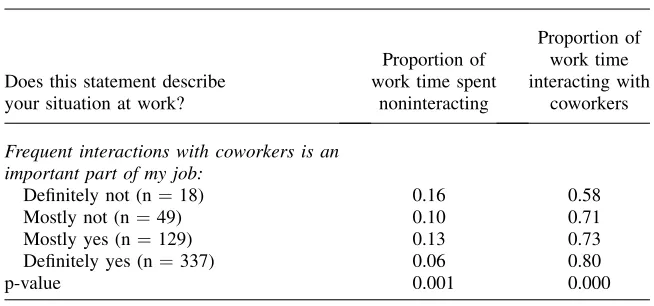
In the Texas DRM we also asked respondents the extent to which the following statement described their situation at work: ‘‘Frequent interactions with coworkers is an important part of my job?’’ Table 2b reports the average proportion of working time involving no interactions, or interactions with coworkers by responses to this job descriptor. Those who answered ‘‘definitely yes’’ spent 80 percent of their
12. We are grateful to Marie Connolly for these tabulations from the ATUS.
Table 1
Descriptive Statistics for the Three Analysis Samples
Texas
All Random Sample Columbus Rennes
Demographic charaterstics
Age 38.0 38.0 43.0 37.9
Annual household income $53,659 $47,915 $69,510 V30,826
Married 0.44 0.42 0.61 0.40
College+a 0.54 0.38 0.55 0.43
Union 0.20 0.12 NA NA
Tenure 6.30 5.59 NA NA
Black 0.24 0.27 0.17 NA
Hispanic 0.22 0.24 0.01 NA
Activity characteristics
Number of work episodes 4.48 3.70 3.86 3.90
Number of work episodes 9.63 9.88 9.78 11.04
Proportion of time alone wihle workingb 0.08 0.08 0.14 0.23
Proportion of time with friends while not workingb 0.44 0.43 0.32 0.33
Proportion of time with friends while not working 0.15 0.16 0.11 0.11
Proportion of interacting while workingc 0.89 0.89 NA NA
Proportion of time conversing while working NA NA NA NA
Maximum sample size 908 535 409 372
Notes: a. In France, college+ is baccalaure´at plus 3 or more years.
b. In Texas, time alone is time spent not interacting with anyone; in Columbus and Rennes, it is time spent alone. c. Proportion of time interacting with customers, clients, cowokers, boss patients or students.
866
The
Journal
of
Human
working time on the reference day interacting with coworkers, while those who an-swered ‘‘definitely not’’ spent 58 percent of their time interacting with coworkers.
Together, these results give us some reason to believe that our time-use measures do reflect social engagement during individuals’ work and nonwork activities.
IV. Empirical Results on Sorting
A. Texas DRM
Table 3 reports estimates of Tobit models where the dependent variable is the pro-portion of time spent interacting at work using the Texas DRM sample. The statis-tical model allows for censoring at zero or one. The key explanatory variable is the proportion of time that the individual was not interacting with someone else dur-ing nonwork episodes (Columns 1 and 2), or the proportion of time the individual was interacting with a friend during nonwork episodes (Columns 3 and 4). Either measure of a person’s ‘‘sociability off work’’ has the expected relationship with the amount of time spent interacting at work.13The effects are also sizable: A 10 percentage point increase in the share of time spent interacting while not working is associated with a 5 percentage point increase in the share of time interacting at work in Column 1.
Variables such as education, marital status, age, and tenure are included as explan-atory variables in Columns 2 and 4. The rationale for including these variables is that they may be related to worker productivity, and sorting by tastes is predicted to take place among workers who are equally productive. For purposes of estimating the ex-tent of sorting, however, it is unclear whether all of these variables should be held
Table 2a
NonWork Time Allocation by Self-Described Gregariousness
What would the people who know you say about you?
Proportion of nonwork time spent noninteracting
Proportion of nonwork time spent with friends
Enjoys being in company:
Much less than others (n¼50) 0.51 0.09
About average (n¼75) 0.42 0.14
Much more than others (n¼390) 0.43 0.17
p-value 0.106 0.017
Note: p-value is from a regression of percent of time reported in each category on self-reported enjoyment from being in company, which runs from23 to +3. Sample is Texas DRM, random sample.
13. If we restrict the sample to those who said the reference day was a typical day, the coefficient on non-interacting time in Columns 1 and 2 tends to rise while the coefficient on interaction time with friends in Columns 3 and 4 tends to fall. In neither case is the qualitative conclusion different, however.
constant. For example, suppose marriage is unrelated to productivity for women, but more gregarious women are more likely to become married (and also more likely to interact with someone off the job) and more likely to work on a job that requires so-cial interaction.14In this case, we would be overcontrolling for tastes. Nonetheless, we find that our proxies for sociability off work remain significantly related to the extent of social interactions on the job despite controlling for the effects of these other variables.
Age is of particular interest because individuals’ may become more or less extro-verted over time. Interactions at home and at work both fall with age. One concern is that people may become more extroverted over time if they are employed in a job that requires interactions. If we interact age with proportion of time not interacting or spent with a friend while away from work we get mixed results, however. Both interaction terms are negative, but neither is statistically significant.
Some of the additional variables are of interest for their own sake. Hispanic work-ers spend about 25 percent less of their working time interacting with othwork-ers than do non-Hispanic workers. Controlling for 19 occupation dummies has no effect on this differential. This finding may, in part, be a manifestation of language differences that reduce communication opportunities for Hispanics at work. Unfortunately, we did not collect information on facility with English. More than language may be at work, however, because we also find that Hispanics are less likely than non-Hispanics to spend time interacting with friends or others off work, where they presumably could interact with Spanish speakers.
Table 2b
Work Time Allocation by Self-Reported Job Description
Does this statement describe your situation at work?
Proportion of work time spent
noninteracting
Proportion of work time interacting with
coworkers
Frequent interactions with coworkers is an important part of my job:
Definitely not (n¼18) 0.16 0.58
Mostly not (n¼49) 0.10 0.71
Mostly yes (n ¼129) 0.13 0.73
Definitely yes (n¼337) 0.06 0.80
p-value 0.001 0.000
Note: p-value is from a regression of percent of time on reported in each category on self-reported job de-scription, which runs from 1 to 4. Sample is Texas DRM, random sample.
Table 3
Tobit Models for Proportion of time Spent Interacting at Work Texas DRM Sample, Random Component
Explanatory Variable (1) (2) (3) (4)
Proportion of time not interacting while not working 20.472 20.395 — —
(0.146) (0.154)
Proportion of time interacting with friend(s) while not working
— — 0.533 0.522
(0.214) (0.225)
Age — 20.007 — 20.008
(0.004) (0.004)
College + — 20.047 — 20.102
(0.084) (0.086)
Married — 0.084 — 0.140
(0.082) (0.083)
Black — 20.113 — 20.104
(0.098) (0.099)
Hispanic — 20.281 — 20.257
(0.099) (0.100)
Union — 20.151 — 20.167
(0.114) (0.116)
Tenure — 20.011 — 20.011
(0.006) (0.006)
Log likelihood 2337.229 2303.426 2339.234 2304.024
Sample Size 534 502 534 502
Note: Dependent variable is proportion of time interacting with coworkers, clients, students, patients, or boss while working. Tobit allows for censoring at 0 and at 1. Mean (SD) of dependent variable is 0.89 (0.24) in Columns 1 and 3, and 0.90 (0.24) in Columns 2 and 4. In Columns 1 and 3, 19 observations are censored at 0, 129 are uncensored and 386 are censored at 1. In Columns 2 and 4, 17 observations are censored at 0, 120 are uncensored and 365 are censored at 1.
Kruege
r
and
Schkade
Union members also spend less time interacting with others at work than do non-union members. Unlike Hispanic workers, however, non-union members are not less likely to interact with friends or others when they are off work. The lower proportion of work time spent interacting by union members may partially explain why union members typically report lower job satisfaction than nonunion members, a phenom-enon first documented by Freeman (1978). Work interactions tend to decline with company tenure, while time interacting with others away from work is unrelated to tenure. Lastly, older workers are less likely to interact with others while working and while not working.
We have also looked at the extent of interaction during work episodes by occupa-tion, assigning 19 two-digit Census occupation codes to the data. An F-test of the null hypothesis that occupation dummies jointly have no predictive power for the proportion of time spent interacting at work has a p-value of 0.026. Because the sam-ple sizes are small, however, the occupational estimates are very imprecise and the results should be taken with a large grain of salt. With that caveat in mind, we find that the legal profession (which includes legal support jobs) and healthcare practi-tioners have the highest rates of interaction at work for an occupation with more than 20 observations, which seems plausible.
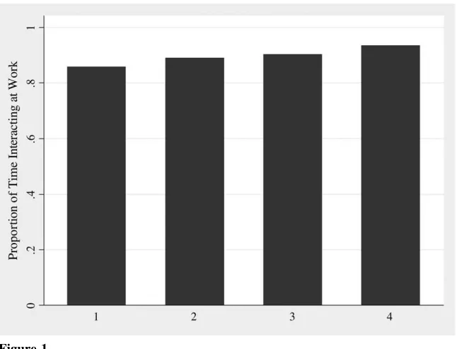
To provide an independent assessment of the extent to which jobs involve social interactions, we assigned each worker an occupation code based on her description of her job and matched the data to theO*NET Dictionary of Occupational Titles. The
O*NETcontains detailed descriptions of the work involved in various occupations. We focus specifically on theO*NETmeasure, ‘‘contact with others,’’ which meas-ures from 0 to 100,‘‘How much does this job require the worker to be in contact with others (face-to-face, by telephone, or otherwise) in order to perform it?’’ For exam-ple, kindergarten teachers were rated a ‘‘contact with others’’ score of 95, statisti-cians were rated a score of 69, and product safety engineers were rated a score of 28. Figure 1 presents the average proportion of work time spent interacting by quartile of the ‘‘contact with others’’ occupational score matched fromO*NET. Despite the crudeness of the data, there is a tendency for workers who are in jobs that are ranked as involving more contact with others to spend more time interacting with others while they are working. The correlation at the individual level is 0.10 (p < 0.01), which is not overwhelming but nonetheless suggests that workers who are on jobs that involve more contact with others tend to spend more of their work time interact-ing with others. We similarly find that workers who are in occupations that involve more contact with others according toO*NETare less likely to be alone while they are at work.
B. French-American Data
Next we consider the data from Columbus, Ohio, and Rennes, France. Two-limit To-bit models for the proportion of time spent talking or engaged in conversation during work episodes are presented in Table 4a for Columbus and Table 4b for Rennes. A test of the hypothesis that the two samples can be pooled is rejected for each model at the 0.01 level.
attenuated when demographic variables are included in the model in Column 2, es-pecially marital status, but, as mentioned, marital status may be related to workers’ gregariousness. The fraction of time spent interacting with friends has a positive ef-fect on interactions at work that is almost statistically significant for the Columbus sample, but it is small and insignificant in the Rennes sample. In Columbus, we find an even larger gap in interactions at work for Hispanic workers15than we found for the Texas sample, although this result should be treated extremely cautiously given that there were only six Hispanic workers in the Columbus sample. We also find that married workers are more likely to engage in conversations while working.16
Unlike in the simple model of sorting that was used to motivate this paper and our estimates so far, workers’ tastes are not unidimensional. It is possible that workers
Figure 1
Proportion of work time spent interacting by quartile of the O*NET‘‘contact with others’’ measure Quartile of job’s ‘‘contact with others’’
Note: Average proportion of time respondents spent interacting with coworkers, customers, clients, students, patients or their boss during episodes that involved work is calculated from Texas DRM. Quartile of ‘‘contact with others’’ is based on linking the full DRM sample to theO*NET Dictionary of Occupational Titles, Third Editionbased on occupational titles. Weighted averages are presented.
15. In France it is illegal to collect ethnicity information and thus we have no comparable results for the Rennes sample.
16. While not working, married women in both Columbus and Rennes spend 17 percent less of their time alone than do single women. At the same time, married women spend 6 percent less of their nonwork time with friends than do single women in Columbus, and 7 percent less in Rennes.
who have a preference for social interactions may also have preferences over other working conditions. Depending on the variance of preferences and the correlation among workers’ preferences, one does not necessarily have to find hierarchical sort-ing along tastes for extroversion and the social nature of jobs. The Columbus and Rennes data sets include a large set of other self-reported preference-type variables. As a partial check on the sensitivity of our results to controlling for a wider set of work-ers’ preferences, in results not shown here we included the workwork-ers’ self-reported plea-sure and joy on a three-point scale (‘‘little or none,’’ ‘‘some,’’ and ‘‘a lot’’) from reading, spiritual and religious life, art, food and eating, nature, television, and taking walks. These variables were jointly statistically insignificant when they were included in each of the models in Tables 4a and 4b, and their inclusion hardly changed the magnitude of the off-work extroversion measures. Thus, controlling for these limited measures of preferences over other attributes that might be related to some jobs does not appear to alter the pattern of sorting by tendency toward extroversion.
A final point worth noting is that despite the greater extent of government inter-vention in the French than in the American labor market, and the higher rate of unionization in France, there is no sign in these results that sorting in the labor mar-ket along lines of the propensity for social interactions is less efficient in Rennes than in Columbus. If this finding can be replicated in other data sets, it could provide insights into the workings of labor market rigidities and comparative labor market institutions.
C. Limits of One Working Day
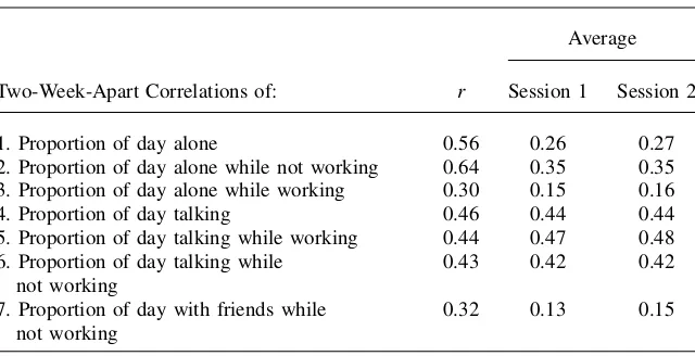
A potential concern is that the data we use to estimate the extent of social interactions by workers while they are working and not working are noisy because the data pertain to just one day in the life of the individuals in the sample. How representative is one work-ing day? To assess this question, we analyzed a sample of 207 women who worked on both reference days in the reliability sample. The version of the DRM used in these sur-veys is virtually identical to that used in the Columbus and Rennes sursur-veys.
Table 4a
Tobit Models for Proportion of Time Spent Interacting at Work, Columbus DRM Sample
Explanatory Variable (1) (2) (3) (4)
Proportion of time alone while not working 20.286 20.136 — —
(0.175) (0.188)
Proportion of time interacting with friend(s) while not working
— — 0.447 0.449
(0.294) (0.300)
Age — 20.003 — 20.003
(0.005) (0.005)
College + — 0.072 — 0.078
(0.099) (0.098)
Married — 0.204 — 0.247
(0.115) (0.108)
Black — 0.256 — 0.250
(0.141) (0.140)
Hispanic — 20.796 — 20.807
(0.453) (0.453)
Log likelihood 2435.01 2425.489 2435.187 2425.625
Sample size 408 403 408 403
Note: Dependent variable is proportion of time talking or engaged in conversation while working. Tobit allows for censoring at 0 and at 1. Mean (SD) of dependent vari-able is 0.44 (0.42) in Columns 1–4; in Columns 1 and 3, 147 observations are censored at 0, 168 are uncensored and 93 are censored at 1; in Columns 2 & 4, 145 obser-vations are censored at 0, 166 are uncensored and 92 are censored at 1.
Kruege
r
and
Schkade
Table 4b
Tobit Models for Proportion of Time Spent Interacting at Work, Rennes DRM Sample
Explanatory Variable (1) (2) (3) (4)
Proportion of time alone while not working 20.467 20.311 — —
(0.202) (0.216)
Proportion of time interacting with friend(s) while not working
— — 0.054 0.166
(0.272) (0.288)
Age — 20.003 — 20.003
(0.005) (0.005)
College + — 20.065 — 20.075
(0.100) (0.100)
Married — 0.204 — 0.266
(0.112) (0.106)
Log likelihood 2367.07 2363.868 2369.752 2364.743
Sample size 371 369 371 369
Note: Dependent variable is proportion of time talking or engaged in conversation while working. Tobit allows for censoring at 0 and at 1. Mean (SD) of dependent variable is 0.34 (0.39) in Columns 1–4; in Columns 1 and 3, 172 observations are censored at 0, 148 are uncensored and 51 are censored at 1; in Columns 2 and 4, 171 are censored at 0, 147 are uncensored and 51 are censored at 1.
874
The
Journal
of
Human
Data Set and regressed the average proportion of time talking during work episodes on the average proportion of time spent with friends during nonwork episodes. The slope coefficient from this bivariate regression is 0.342 with a standard error of 0.156.17If the same regression is estimated just using Session 1 data, the coefficient (standard error) is 0.273 (0.149) and if it is estimated for Session 2 the coefficient (stan-dard error) is 0.224 (0.149). If the first period proportion of time spent with friends is used as an instrument for the second period proportion of time with friends in an instru-mental variables regression that uses the second period proportion of time talking at work as the dependent variable, the coefficient is considerably larger: 1.003 (0.493). All of these results suggest that noise has attenuated our earlier estimates.
An alternative way to avoid relying on one day’s measures is to use individual’s own descriptions of their jobs and personalities. As was shown in Tables 2a and 2b, these measures are correlated with objective circumstances on and off the job. If we use the Texas DRM data to regress individuals’ assessments of whether, ‘‘Fre-quent interactions with coworkers is an important part of my job?’’ on their assess-ments of whether people they know would say that they enjoy being in the company of others, we find a significant and positive relationship (r¼0.11;p¼0.01). Reliance on self-reported personality and job traits is common in the personnel selection lit-erature. We consider a focus on actual time allocation to be a contribution of our study, but it is nonetheless reassuring that we find sorting based on a tendency for extroversion when we use self-reported data as well.
Table 5
Reliability of Data
Average
Two-Week-Apart Correlations of: r Session 1 Session 2
1. Proportion of day alone 0.56 0.26 0.27
2. Proportion of day alone while not working 0.64 0.35 0.35
3. Proportion of day alone while working 0.30 0.15 0.16
4. Proportion of day talking 0.46 0.44 0.44
5. Proportion of day talking while working 0.44 0.47 0.48 6. Proportion of day talking while
not working
0.43 0.42 0.42
7. Proportion of day with friends while not working
0.32 0.13 0.15
Notes: Sample consists of 207 women in Texas who were sampled on March 30 and April 13, 2005 and worked on the preceding day. Both surveys were conducted on a Wednesday, and the responses refer to the preceding day. The average respondent reported 9.7 nonworking episodes and 4.6 working episodes per day. The definition of the variables conforms to those used in the Columbus and Rennes DRM samples.
17. If we use the average amount of time spent alone while not working as the explanatory variable, the coefficient (standard error) is20.115 (0.101).
V. Work Satisfaction and Affect at Work
We measure individuals’net affector mood as the average of the pos-itive emotions less the average of the negative emotions recorded for each episode in the DRM. Emotions are reported on a scale of zero (not at all) to six (very much part of the experience). Positive emotions are ‘‘happy’’ and ‘‘enjoying myself’’ and neg-ative emotions are ‘‘impatient for it to end,’’ ‘‘frustrated/ annoyed,’’ ‘‘depressed/ blue,’’ ‘‘worried/anxious,’’ and ‘‘angry/hostile.’’ These emotions were selected be-cause they do not necessarily require social interaction to be present.
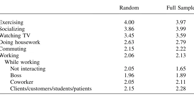
Table 6 reports average net affect during episodes that involved selected work and nonwork activities for the full sample and random subsample of the Texas DRM sur-vey. Notice that, on average, work is ranked as a relatively unpleasant activity and leisure activities such as socializing and exercising have relatively high net affect rat-ings. This pattern is not surprising—and, indeed, presumably it is the reason why wages are positive—but it contrasts with earlier research based on more general questions about enjoyment with various activities (Juster 1985; Robinson and God-bey 1997). Juster (1985), for example, finds that work ranks near the middle of ac-tivities in terms of enjoyment. The difference appears to stem from our using a recall diary method as opposed to Juster’s use of an overall domain satisfaction approach, in which people’s subjective theories about their lives probably play a larger role.
Average net affect during work episodes that involve interactions with the boss is particularly low, while net affect is higher during interactions with customers, clients, students, or patients. Workers in the full sample report especially low affect when they are working alone. All of the averages in Table 6 are potentially affected by sort-ing, as not every worker engaged in each activity.
Another limitation of self-reported feelings like those in Table 6 is that respondents may utilize the scales in idiosyncratic ways. We therefore examined the pattern of net affect during various types of work interactions after removing individual fixed effects. Specifically, we regressed net affect during each episode on three dummy variables in-dicating whether that episode involved an interaction with the boss, coworkers, or cli-ents, customers, studcli-ents, and paticli-ents, and a set of unrestricted individual fixed effects. This fixed effects model is identified by workers who had at least one work episode in-volving social interactions and at least one work episode without interactions on the sur-vey reference day. Within a person’s work day, we find that interactions have a large effect on net affect. For the random sample, compared with not interacting with anyone, net affect was 0.53 (0.14) points lower when an episode involved interacting with the boss, 0.24 (0.12) points higher when coworkers were interaction partners and 0.40 (0.18) points higher when customers, clients, students, or patients were involved.
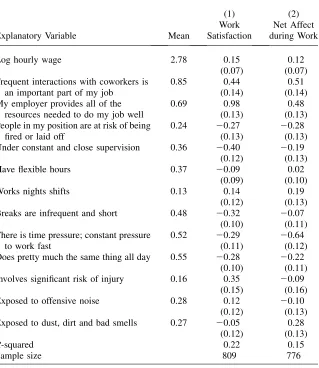
Table 7 presents estimates of regression models at theindividuallevel using the Texas DRM sample.18The dependent variable in Column 1 is responses to a conven-tional work satisfaction question: ‘‘Overall, how satisfied are you with your present job?’’ Response categories were not at all satisfied, not very satisfied, satisfied, and very satisfied. A score from one to four was assigned to these answers, and then the responses were rescaled to have a unit standard deviation. Many previous studies (Freeman 1978;
18. To increase the sample size, results are reported for the full sample. If we restrict the data to the random subset, however, the main results are qualitatively similar.
Helliwell and Huang 2005; Green, 2006) have examined the determinants of global work satisfaction. The dependent variable in Column 2 is duration-weighted net affect while at work. This measure should provide a closer approximation of workers’ actual emotional experiences on the job than reported work satisfaction. Net affect is com-posed of the same emotions as in Table 6. For comparability to work satisfaction, net affect was rescaled to have a unit standard deviation in the regressions.
A rich set of working condition variables is available to model subjective well-be-ing at work. Table 7 reports results uswell-be-ing a dozen workwell-be-ing conditions as explanatory variables, including the extent to which the respondent stated that her situation at work was described by ‘‘frequent interactions with coworkers,’’ ‘‘constant and close supervision,’’ and ‘‘flexible work hours.’’ Four responses categories ranging from ‘‘definitely not’’ to ‘‘definitely yes’’ were provided, and answers were scaled from zero to one, with zero indicating definitely not and one indicating definitely yes. Thus, the coefficients indicate the change in work satisfaction or net affect in stan-dard deviation units associated with a change from the working condition being def-initely absent to defdef-initely present. The regression models also control for the log hourly wage, education, and demographic characteristics.
The working condition variables generally have their expected signs, although there are a few notable exceptions. Most importantly for our purposes, having a job that allows frequent interactions with coworkers is positively associated with work satisfaction and with net affect while at work, conditional on the sorting that takes place in the job market. Workers who believe their job entails frequent inter-actions with coworkers report about half a standard deviation higher work satisfac-tion and net affect than do those who say their job does not entail frequent
Table 6
Net Affect During Various Activities; Texas DRM Sample
Random Full Sample
Exercising 4.00 3.97
Socializing 3.86 3.99
Watching TV 3.45 3.59
Doing housework 2.63 2.79
Commuting 2.15 2.22
Working 2.06 2.13
While working
Not interacting 2.05 1.65
Boss 1.96 1.89
Coworker 2.05 2.11
Clients/customers/students/patients 2.15 2.28
Notes: Averages are reported for the random sample and for the full sample from the Texas DRM. Net af-fect is the difference between the duration-weighted average of positive emotions (‘‘happy’’ and ‘‘enjoying myself’’) and the duration-weighted average of negative emotions (‘‘impatient for it to end’’, ‘‘frustrated/ annoyed’’, ‘‘depressed/blue’’, ‘‘worried/anxious’’ and ‘‘angry/hostile’’).
interactions. From our earlier results and Equation 1, we would expect that workers who receive greater enjoyment from social interactions would be more likely to be employed in jobs that require frequent interactions with others. To test directly for this result, in results not shown here we added a variable that is the product of the frequent-job-interaction variable and the proportion of nonwork time each re-spondent spent alone (based on their time diary) to the regression models. The
Table 7 resources needed to do my job well
0.69 0.98 0.48
(0.13) (0.13)
People in my position are at risk of being fired or laid off
0.24 20.27 20.28
(0.13) (0.13)
Under constant and close supervision 0.36 20.40 20.19
(0.12) (0.13)
Have flexible hours 0.37 20.09 0.02
(0.09) (0.10)
Works nights shifts 0.13 0.14 0.19
(0.12) (0.13)
Breaks are infrequent and short 0.48 20.32 20.07
(0.10) (0.11)
There is time pressure; constant pressure to work fast
0.52 20.29 20.64
(0.11) (0.12)
Does pretty much the same thing all day 0.55 20.28 20.22
(0.10) (0.11)
Involves significant risk of injury 0.16 0.35 20.09
(0.15) (0.16)
Exposed to offensive noise 0.28 0.12 20.10
(0.12) (0.13)
Exposed to dust, dirt and bad smells 0.27 20.05 0.28
(0.12) (0.13)
R-squared 0.22 0.15
Sample size 809 776
Notes: Regressions also include a constant, education, age, age-squared, and Hispanic ethnicity, black, and white indicator variables. Standard error shown in parentheses. Work satisfaction and net affect have been scaled to have a standard deviation of 1.
coefficient on this interaction variable was -0.34 and statistically significant (t¼2.29) in the net affect regression, consistent with the view that more social workers derive more enjoyment from jobs that entail frequent interactions with coworkers.19The in-teraction effect was negative but small and statistically insignificant in the work sat-isfaction model, however.
Turning to the other variables in Table 7, the log wage has a positive effect on both work satisfaction and net affect at work. A 10 percent increase in pay is associated with just over a 0.015 standard deviation gain in work satisfaction, which is fairly modest compared with the effects of several of the working condition variables, in-cluding interactions with coworkers. Time pressure, close supervision, risk of job loss, and monotony all have sizable adverse effects on work satisfaction and on net affect during work. Reporting that one’s employer provides all the resources needed to do the job well has a strong positive effect on satisfaction and net affect. Although there is some tendency for working conditions that have an immediate and salient effect on the work setting, like time pressure, to have a larger effect on net affect than on work satisfaction, this is not always the case. For example, constant and close supervision has a larger effect on work satisfaction than on net affect, as does belief that sufficient resources are provided to do the job well.
Some of the working condition variables in Table 7 have statistically insignificant effects, such as flexible hours and the presence of offensive noise. Two notable var-iables have perverse effects: The presence of dust, dirt, and bad smells has an unex-pected positive effect in the net affect regression and the presence of a risk of injury has a positive effect in the work satisfaction regression. As a whole, however, the models yield reasonably strong support that pleasant working conditions are associ-ated with greater job satisfaction and net affect at work, and unpleasant working con-ditions are associated with lower job satisfaction and net affect at work.
Lastly, it is worth discussing the magnitude and interpretation of the working con-dition effects in relation to an equalizing differences equilibrium in the labor market. Helliwell and Huang (2005) argue that dividing the coefficient on a working condition variable by the coefficient on the wage rate in a job satisfaction regression provides an estimate of the marginal rate of substitution between log pay and working conditions. If workers have homogeneous preferences, in a competitive equilibrium this ratio would equal the observed compensating wage differentials associated with working conditions. Using this approach, Helliwell and Huang find that enormous compensat-ing wage differentials are required for workcompensat-ing conditions such as low workplace trust, low task variety, and time pressure. Because direct evidence of compensating wage differentials often yields mixed or weak evidence of tradeoffs between pay and work-ing conditions (see Brown 1980),20Helliwell and Huang conclude that the labor mar-ket is in disequilibrium, with ‘‘unrecognized opportunities for managers and employees to alter workplace environments, or for workers to change jobs, so as to increase both life satisfaction and workplace efficiency.’’
19. It is worth noting that in this regression, workers who spent all of their nonwork time alone were pre-dicted to have higher net affect if their jobs entailed frequent interactions with coworkers than if they did not entail frequent interactions with coworkers.
20. One recent exception is Stern (2004), who finds a sizable tradeoff between the opportunity to conduct and publish scientific research and starting pay among Ph.D. biologists at the start of their career.
Our results also imply an enormous tradeoff between wages and undesirable work-ing conditions. For example, the results in Column 1 of Table 7 imply that workers would require a log wage increase of around two (20.29/0.15) to be equally satisfied with a job that entails constant time pressure as opposed to one that does not. The net affect regression in Column 2 implies a log wage change of more than five for work-ers to be equally well-off with constant time pressure. Moving from a job with fre-quent interactions with coworkers to one without them likewise would necessitate large compensating payments, as would many of the other working conditions.
What is one to make of Helliwell and Huang’s and our large implied marginal rates of substitution? One possibility is that job satisfaction is not an adequate mea-sure of utility because it misrepresents what happens on the ground at work. The fact that net affect generally yields similar results, however, suggests that the explanation is more complicated.
Another possibility is that the coefficients in the work satisfaction and net affect regressions reflect the preferences of inframarginal workers while the compensating differentials that are ground out in practice pertain to the preferences of the marginal worker. This distinction matters if tastes vary across workers and workers sort into jobs based on their tastes, as we have emphasized. Regression estimates like those in Table 7 only identify conditional averages, and the averages are conditional on the workers sorting. The marginal worker probably has a more benign view of social isolation than the average worker in a job that does not involve interactions with coworkers, for example. While we believe there is some support for this interpreta-tion, the results imply that such extreme compensating differentials are required for undesirable working conditions that we would question how far sorting by preferen-ces can go toward explaining the full set of results.
Still another possibility is that direct estimates of compensating wage differentials suffer from severe biases. For example, high-ability workers receive higher pay and bet-ter working conditions than low-ability workers, but the estimates in the libet-terature may not adequately control for ability. While this bias is likely present in cross-sectional estimates, it is unlikely to account for the weak evidence of compensating wage entials in longitudinal estimates. Moreover, if the required compensating wage differ-entials are as large as those implied in Helliwell and Huang and in Table 7, we would expect that they would be detectable in conventional wage equation estimates.
A final interpretation is that the marginal worker is unaware of the relevant working conditions when a decision is made to accept a job, or underestimates the impact of social relations and other working conditions on her well-being and overestimates the impact of pay on her well-being, perhaps because of a focusing illusion (see Kahne-manet al.2006). In either case, this failure of decision making would cause the market to generate insufficient compensating differentials for working conditions. Although we are reluctant to push this conclusion too far, given the similarity of the results using job satisfaction and net affect, we believe it deserves serious consideration.
VI. Conclusion
while not working and the relative frequency of work-related interactions on the worker’s job. We interpret this pattern as evidence of sorting: more extroverted work-ers tend to work in jobs that require greater social interaction.
Other interpretations are possible, however. For example, it is possible that jobs that require more social interactions cause workers to become more extroverted in their nonworking time. Although extroversion is apparently among the more stable personality traits (Roberts and DelVecchio 2000) and Borghans, ter Weel and Wein-berg (2006a, 2006b) find that sociability at an early age is related to later employ-ment in occupations that involve more people skills, we acknowledge that work experiences could affect an individual’s tendency to extroversion. It is also possible that a tendency towards extroversion causes some workers to spend a lot of time interacting with others while away from work and while at work, but that the social interactions during work time are not work related. While we acknowledge this pos-sibility, our finding of a positive correlation between work time spent interacting with others and the contact score for the job based on theO*NET Dictionary of Occupa-tional Titlessuggests that extroverted workers are more likely than introverted work-ers to be employed in positions that utilize social skills.
Biasing our results in the opposite direction, one should also recognize that many workers who spend their entire work day talking might seek some solitude when they are off work. This effect, if it exists, is not strong enough to overturn the positive relationship between the prevalence of work-related and nonwork-related interac-tions.
Another concern is that workers’ tastes are not unidimensional. It is possible that workers’ who have a preference for social interactions may also have preferences over other working conditions. A worthwhile direction for future work would be to develop measures of tastes toward other work-related conditions, such as risk, of-fensive noise, and stress, and then to jointly test whether sorting occurs on jobs along those lines as well extroversion. For example, the seemingly anomalous results we found for risk and offensive noise may be due to occupations such as hospital nurses or construction workers, whose jobs involve these negative characteristics, but which are outweighed by other positive features. Multidimensional sorting could well re-solve these puzzling results.
Competitive markets are presumed to raise welfare by enabling buyers and sellers, workers and employers, to make efficient matches according to their tastes, talents, and technology. The extent to which workers are actually sorted across jobs accord-ing to their tastes has not previously been examined. An important feature of our work is that we identify workers’ tastes toward social interactions by their revealed behavior while not working. Similar results are found, however, if we use self-reported indicators of individuals’ personality traits.
The approach we have taken can be used to compare the efficiency of different labor markets. Although our evidence is admittedly sketchy and preliminary – and dependent on the assumption that opportunities for socializing while not working are similar in the two countries – we do not find much evidence of differential sorting by workers’ preferences for social interactions in France and the United States. If correct, this finding suggests that the rigidities in the French labor market do not ob-struct the efficient sorting of workers across jobs in a noticeable way. A useful direc-tion for future work would be to examine the extent to which the matching of
workers and jobs according to workers’ tastes are affected by labor market institu-tions.
Lastly, we find that workers express higher levels of satisfaction and higher net affect during work if they are employed in jobs that involve frequent interactions with coworkers. This effect tends to diminish for workers who spend a smaller share of their nonwork day in the company of others. We also find that other workplace characteristics, such as time pressure, close supervision, and perceived risk of job loss, have a sizable effect on work satisfaction and net affect on the job. The esti-mated effect of desirable working conditions on work satisfaction and net affect is especially large in comparison with the modest estimated effect of pay on work sat-isfaction and net affect, and the typically modest compensating wage differentials as-sociated with various working conditions observed in the labor market. The reasons for this divergence deserve further consideration.
References
Borghans, Lex, Bas ter Weel, and Bruce Weinberg. 2006a. ‘‘People People: Social Capital and the Labor-Market Outcomes of Underrepresented Groups.’’ National Bureau of Economics Research Working Paper 11985.
__________. 2006b. ‘‘Interpersonal Styles and Labor Market Outcomes.’’ Maastricht University. Unpublished.
Brown, Charles. 1980. ‘‘Equalizing Differences in the Labor Market.’’Quarterly Journal of Economics94(1):113–34.
Freeman, Richard. 1978. ‘‘Job Satisfaction as an Economic Variable.’’American Economic Review68(2):135–41.
Green, Francis. 2006.Demanding Work.Princeton: Princeton University Press. Gronau, Reuben. 1974. ‘‘Wage Comparisons—A Selectivity Bias,’’Journal of Political
Economy82(6):1119–43.
Hamermesh, Daniel. 1990. ‘‘Shirking or Productive Schmoozing: Wages and the Allocation of Time at Work.’’Industrial & Labor Relations Review43(3):121–33.
Helliwell, John, and Haifang Huang. 2005. ‘‘How’s the Job? Well-Being and Social Capital in the Workplace.’’ National Bureau of Economics Research Working Paper 11759. Hough, Leaetta, and Frederick Oswald. 2000. ‘‘Personnel Selection: Looking Toward the
Future—Remembering the Past.’’Annual Review of Psychology51:631–64.
Juster, F. Thomas. 1985. ‘‘Preferences for work and leisure’’. InTime, Goods, and Well-being, ed. F. Thomas Juster and Frank Stafford, 335–51. Ann Arbor: Institute for Social Research, University of Michigan.
Kahneman, Daniel, Alan Krueger, David Schkade, Norbert Schwarz and Arthur Stone. 2004. ‘‘A Survey Method for Characterizing Daily Life Experience: The Day Reconstruction Method (DRM).’’Science306(5702):1776–80.
__________. 2006. ‘‘Would You Be Happier If You Were Richer? A Focusing Illusion.’’
Science312(5782):1908–10.
Krueger, Alan, and David Schkade. 2008. ‘‘The Reliability of Subjective Well Being Measures.’’Journal of Public Economics92(8-9):1833–45.
Roberts, Brent, and Wendy F. DelVecchio. 2000. ‘‘The Rank-Order Consistency of Personality Traits from Childhood to Old Age: A Quantitative Review of Longitudinal Studies.’’Psychological Bulletin126(1):3–25.
Robinson, John, and Geoffrey Godbey. 1997.Time for Life: The Surprising Ways Americans Use Their Time.University Park, Pennsylvania: The Pennsylvania State University Press. Rosen, Sherwin. 1986. ‘‘The Theory of Equalizing Differences.’’Handbook of Labor
Economics, volume 1, ed. Orley Ashenfelter and Richard Layard, 641–92. Amsterdam: North Holland.
Rosen, Sherwin. 2002. ‘‘Markets and Diversity.’’American Economic Review92(1):1–15. Saffer, Henry. 2005. ‘‘The Demand for Social Interactions.’’ National Bureau of Economics
Research Working Paper 11881.
Stern, Scott. 2004. ‘‘Do Scientists Pay To Be Scientists?’’Management Science50(6): 835–53.
Tinbergen, Jan. 1956. ‘‘On the Theory of Income Distribution,’’Weltwirtschaftliches Archiv
77:155–75.
Viscusi, Kip, and Joni Hersch. 2000. ‘‘Cigarette Smokers as Job Risk Takers.’’Review of Economics and Statistics83(2):269–80.