STOCHASTIC TWO-STAGE PROGRAM
APPROACH FOR MULTI OBJECTIVE SUPPLY
CHAIN DESIGN TO CONSIDER FINANCIAL
RISK
Siti Fatimah Sihotang, Dame Meldaria Sipahutar, Saib Suwilo
Abstract. Many mathematical problem can be solved by stochastic program. Stochastic program aims to determine a feasible solution model when there is a problem in the matter of uncertainty. Supply chain management is one of the cases that are used to manage the condition of uncertainty. Uncertainty can be a production - distribution planning, customer satisfaction, the number of demand, the number of supply, transportation costs, shortage costs, capacity expansion costs, until on the problem of financial risk. In order to consider the effect of uncertainty in these scenarios, two-stage stochastic program model is proposed in this research. Two-stage stochastic program model, paired with the concept of multi objective. Therefore, this research aimed to develop a two-stage stochastic program model with the concept of multi objective to solve supply chain design problems which considering the financial risk.
1. INTRODUCTION
Application of the supply chain is considered increasingly important in to-day’s era of industrialization. A supply chain running smoothly considered ideal and beneficial for those who apply them. Azaron et al. [2] described
Received 15-08-2013, Accepted 15-10-2013.
2010 Mathematics Subject Classification: 90C15, 90C29
Key words and Phrases: Supply chain, Stochastic program multi objective, Risk management.
supply chain is a network of distribution, manufacturing, warehousing and distribution channel organization. Distribution network is used to obtain raw materials, to convert the raw materials to become a product and dis-tribute products to customer.
Meanwhile, supply chain management is a simple business concept to improve the productivity of all companies belonging to the supply chain through the optimization of quality and time. Supply chain management can be used to cope with uncertainty. Thus, many mathematical problems that can be solved by stochastic program. The aim is to determine a viable solution model when in these problems, there are problems of uncertainty. This is consistent with that proposed by Birge and Louveaux [5], many problems of optimization containing uncertainty.
The used method in this study to model the supply chain design prob-lem is the allocation of a two-stage method paired with the concept multi objective. The concept of multi objective used for representing the issue of supply chain design that allows for two or more objective functions.
Here are presented some researches that focus on issues - strategic and tactical issues simultaneously for supply chain design using two-stage stochastic model paired with the concept of multi objective. Azaron et al. [2] using a stochastic program approach based on recursive two-stage models. This approach combines the uncertainty associated with demand, supply, processing costs, transportation costs, cost disadvantages, and the cost of the expansion of capacity. To develop robust models, two additional objective functions are added in the supply chain design problem.
Meanwhile, Mirzapouret al.[8] also apply a two-stage stochastic pro-gram multi objective on supply chain issues that specifically discusses the planning of production - distribution under uncertainty condition based on risk and worker productivity. Then, in designing a model of the problem, three objective functions are added in this study. In the same year, Alborzi
et al.[1] also conducts research related to supply chain network design con-sisting of several suppliers, some of production plant, distribution centers and small traders, are also be considered. The demand of small traders con-sidered as stochastic parameters, thus constructed a number of data through simulation.
this study relates to a design plan in uncertainty is defined as the probabi-lity of non-fulfillment of a number of specific budget or profit targets which have been set.
2. LITERATURE REVIEW
2.1 Stochastic Program Approach for Supply Chain Design
Many of problems of planning and operational management of uncertainty are discussed and solved by stochastic program. More specifically discussed at a two-stage stochastic program. For example take the case of the design of supply chain problems.
In general, Alborziet al. [1] explains that performance of the supply chain can be classified in two ways, namely qualitative and quantitative supply chain performance. Customer satisfaction, flexibility, and effective risk management categorized as qualitative factors. While the quantitative factors, these factors are categorized by two things:
1. Objectives are based directly on price or profit such as, minimizing price, maximizing profits, etc.
2. Objectives are based on some measure of customer response, such as minimizing response time to customers, minimizing time the order, and etc.
The proposed model in this approach is used to determine the design of the three levels of supply chain (production - warehouse - market) to maximize the calculation of the three objective functions (net present value, demand satisfaction, and risk).
2.2 Definition of Risk
2.3 Definition of Risk Management
Risk management is a systematic way of looking at a risk and determine appropriate risk management. It is a means to identify the sources of risks and uncertainties. It Means to improve the effect and develop responses that must be done to respond the risks. This notion is explained by Uher and Toakley [9].
2.4 Net Present Value (NPV)
Net present value is a value that is used as a direct measure of how well a project investment can achieve as expected. Gregoriouet al.[6] explained a good working capital investment is one that has a positive net present value which aims to increase the wealth of its owner.
According by Barbaro and Bagajewicz [4], deals with the issue of sup-ply chain design, the NPV will be different for each issue. Different NPV value obtained for each scenario studied (N P Vn) after the uncertainty is described.
Therefore, the model described in each issue should describe the ex-pected maximum value (E[NPV]). Its value can be calculated by the NPV is expressed by the following equation:
E[N P V] =X n
probnN P Vn (1)
3. PROBLEM FORMULATION
3.5 Supply Chain Problems
In last decade, development of supply chain into a topic that is important to consider its issue on the international community, especially in the field of automobiles, computers, and industrial. Successful supply chain manage-ment requires an integrated system. Each unit in the supply chain must be a unity, not standing in its own.
planning including on the types of operational activities. These activities do a plan for production process, to give an idea to the management as to what quantity of materials and other resources that will be purchased. As a result, total operational costs organization maintained in order minimum during this period.
3.6 Stochastic Program Model
Stochastic program is a name which states mathematical program that can be linear, natural numbers, a mixture of natural numbers, non-linear but with display a stochastic element in the data. The general form of stochastic program can be written as follows introduced by Kall and Wallace [7]:
min f(x) =cTx= n X
j=1
cjxj (2)
s.t
ATi x= n X
j=1
aijxj ≥bi, i= 1,2, ..., m (3)
xj ≥0, j = 1,2. . . , n (4)
where cj,aij and bi are discrete random variables (variables decision xj in this case assumed to be deterministic) known distribution of probability.
3.7 A Two-Stage Stochastic Program Model
A two-stage stochastic program model is a stochastic problem of conver-sion into an equivalent deterministic problem. Completion of a two-stage stochastic program consists of random and deterministic vectors. At the approach of a two-stage stochastic program model, decision variables are divided into two sections:
1. The group of specified variable before the realization of a random event that is known is referred to as the first stage of decision variables.
2. Another group of variables known as recursive variables are determined after knowing the value of the realization of the random events.
program to completion. It means, for the issue of double stage, the influ-ence of decision now will wait for some of the uncertainty that settled back (realized). With the aim of making another decision will be based on what is happening. The ultimate aim to be achieved is to minimize the expected costs of all decisions taken. General form of a two-stage stochastic program model with a simple recursive can be formulated as follows introduced by Barik et al. [3]:
stage decision variable and second stage decision variables. Furthermore qi,
i= 1,2, . . . , m1 is determined as penalty costs associated with the difference
3.8 Stochastic Two-Stage Program Approach for Multi Ob-jective Supply Chain Design to Consider Financial Risk
Birge and Louveaux [5] described in two-stage stochastic optimization app-roach, the uncertain model parameters are considered as random variables with probability distributions associated. The random variables such deci-sion is based on two stages. After the first stage of the decideci-sion taken and random events are known, the second stage of the decision addressed to the restrictions imposed by the second stage problem. Because of the stochastic nature of the performance associated with the second phase of the decision, the objective function consists of the sum to measure the performance of the first stage and second stage of the expected performance. Models of deterministic mathematical formulation for two-stage stochastic formulated as follows introduced by Azaronet al. [2]:
with constraints
y ǫY ⊆ {0,1}|P|, (10)
where [G(y, ξ)] is the optimum value of the following problems:
min qTx+hTz+fTe (11)
Furthermore, model (9-17) can be expanded by adding the concept of multi objective to supply chain design problem. Multi objective optimiza-tion problem appears in most of the problems of decision making in real life. Therefore, the general form of a the multi objective two-stage stochastic pro-gram model of multi objective stochastic propro-gram model can be written as follows introduced by Bariket al. [3]:
max zt=
Thus, a multi objective two stage stochastic model which appropriate for supply chain design problem can be written as follows introduced by Azaron et al. [2]:
C : Collection of customer centers
S : Collection of suppliers
Y : The set is not empty and limited
c : Investment costs
q : Processing costs / transport
h : Cost per unit incurred for failing to fulfill the demand and supply
x : Flow products supplied
z : Lack of product that has made it impossible for any request
E : Expansion of capacity
f : The cost of each unit expansion
L : Worth with|T|x2|S|states the total number of scenarios, including the case - matters relating to the reliability of the supplier
The first objective function associated with minimizing the total cost of the investment first stage and the processing costs of the second stage are expected, cost of transportation, shortage costs and costs of expanding capacity.
The second objective function associated with minimizing the variance cost of the second stage or the variance of the total cost. Variances should be considered in the model because when only focus on the expected total cost, the design scheme in the supply chain may be sub-optimal.
Therefore, it is necessary to introduce a new objective function to clearly capture the notion of risk (as a result of the calculation of the cost of variance in the previous objective function). The issue of risk is always identical to the uncertainty inherent in any investment that has a relatively long time.
In the case related to the risk, NPV value obtained should be smaller than a predetermined profit targets. This is in accordance with the principle of excess NPV method, this method can take into account the residual value of a job. With these considerations, for the multi objective two-stage stochastic program model (23-32), the issue of supply chain design can add a new objective function, which is related to financial risk. Financial risk is any form of risk associated with financial which having an immediate effect on cost control. In the design of supply chain, financial risk occurs when there is a change in the price of goods and services. Then, coupled with the reputation risk associated with the loss of a good reputation of the company. Therefore, based on the principle of the expected value and risk, to issue a two-stage stochastic program, financial risk can be written relating to the design d and the target profit Ω which can be explained by the following probabilities:
Financial Risk(d,Ω) =P(N P V(d)<Ω) (33)
where N P V(d) is a real advantage that the benefits obtained after the un-certainty has been described and scenarios have been realized.
Definition of financial risk (d,Ω) can be rewritten by the following equation:
Financial Risk(d,Ω) =X n
Thus, an additional objective functions that can be added in the model related to financial risk can be written mathematically, as follows:
Min Z3=
X
n
Xn(d,Ω).Pn (35)
The third objective function related to minimizing financial risk ari-sing from the supply chain design work plan.
4. NUMERICAL EXAMPLE
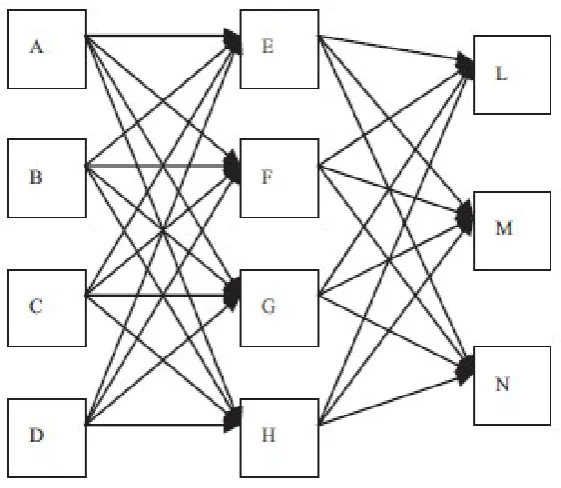
A syrup companies intend to design the supply chain. The company has three customer centers located in three different cities, namely L, M and N. Syrup with qualified uniform in large quantities supplied from four refineries located in A, B, C and D. There are four possible locations to build bottling plant that is E, F, G and H. There is an option to expand the capacity of the bottling plant F, if F bottling plant was built.
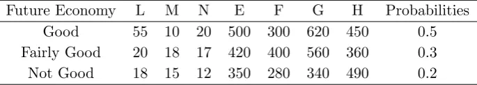
For simplicity, each market demand depends only on local economic conditions. It is assumed that the future state of the economy condition is in three state of the economy. These state, which are in a state of good, fairly good, and in a state that is not good. Three situations have respective probabilities of 0.5; 0.3; 0.2. The production cost per unit is determined in units of rupiah.
Table 1: Characteristic of the problems
Future Economy L M N E F G H Probabilities Good 55 10 20 500 300 620 450 0.5 Fairly Good 20 18 17 420 400 560 360 0.3 Not Good 18 15 12 350 280 340 490 0.2
Specification:
1. The value of L, M, and N in units, which explains the demand.
Market demand based on each scenario are shown in Figure 1 below:
Figure 1: The supply chain design problem of syrup company
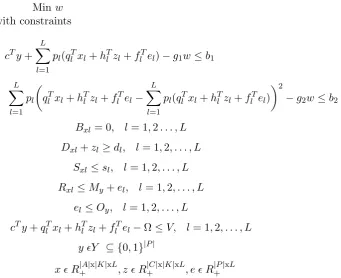
This problem aims to minimize the total expected cost, the variance of total cost, and the financial risk in a multi objective scheme. It also makes the determination of the following problem: ”Which of the bottling plant to be built?”. To solve the problem of multi objective design of the supply chain in this case, used formulation goal attainment which is a variation of goal programming techniques.
Minw
with constraints
cTy+ L X
l=1
pl(qTl xl+hTl zl+flTel)−g1w≤b1
L X
l=1 pl
qlTxl+hTl zl+flTel− L X
l=1
pl(qlTxl+hTl zl+flTel) 2
−g2w≤b2
Bxl = 0, l= 1,2. . . , L
Dxl+zl≥dl, l= 1,2, . . . , L
Sxl≤sl, l= 1,2, . . . , L
Rxl ≤My+el, l= 1,2, . . . , L
el≤Oy, l= 1,2, . . . , L
cTy+qlTxl+hTl zl+flTel−Ω≤V, l= 1,2, . . . , L
y ǫY ⊆ {0,1}|P|
x ǫ R+|A|x|K|xL, z ǫ R+|C|x|K|xL, e ǫ R|P+|xL
Formulation of mathematical models have 9 binary variables, i.e. the num-ber of configurations, g1, g2, b1, b2, Ω, E, F, G, H, mean, variance, and
time. Then, used LINGO 10software to solve the problem and to produce Pareto-optimal solutions numerically different.
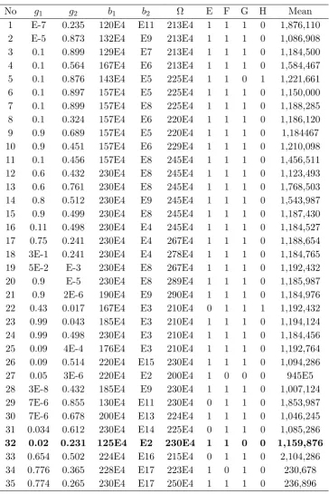
Table 2: Pareto-optimal solution without considering financial risk
No g1 g2 b1 b2 Ω E F G H Mean
1 E-7 0.235 120E4 E11 213E4 1 1 1 0 1,876,110 2 E-5 0.873 132E4 E9 213E4 1 1 1 0 1,086,908 3 0.1 0.899 129E4 E7 213E4 1 1 1 0 1,184,500 4 0.1 0.564 167E4 E6 213E4 1 1 1 0 1,584,467 5 0.1 0.876 143E4 E5 225E4 1 1 0 1 1,221,661 6 0.1 0.897 157E4 E5 225E4 1 1 1 0 1,150,000 7 0.1 0.899 157E4 E8 225E4 1 1 1 0 1,188,285 8 0.1 0.324 157E4 E6 220E4 1 1 1 0 1,186,120 9 0.9 0.689 157E4 E5 220E4 1 1 1 0 1,184467 10 0.9 0.451 157E4 E6 229E4 1 1 1 0 1,210,098 11 0.1 0.456 157E4 E8 245E4 1 1 1 0 1,456,511 12 0.6 0.432 230E4 E8 245E4 1 1 1 0 1,123,493 13 0.6 0.761 230E4 E8 245E4 1 1 1 0 1,768,503 14 0.8 0.512 230E4 E9 245E4 1 1 1 0 1,543,987 15 0.9 0.499 230E4 E8 245E4 1 1 1 0 1,187,430 16 0.11 0.498 230E4 E4 245E4 1 1 1 0 1,184,527 17 0.75 0.241 230E4 E4 267E4 1 1 1 0 1,188,654 18 3E-1 0.241 230E4 E4 278E4 1 1 1 0 1,184,765 19 5E-2 E-3 230E4 E8 267E4 1 1 1 0 1,192,432 20 0.9 E-5 230E4 E8 289E4 1 1 1 0 1,185,987 21 0.9 2E-6 190E4 E9 290E4 1 1 1 0 1,184,976 22 0.43 0.017 167E4 E3 210E4 0 1 1 1 1,192,432 23 0.99 0.043 185E4 E3 210E4 1 1 1 0 1,194,124 24 0.99 0.498 230E4 E3 210E4 1 1 1 0 1,184,456 25 0.09 4E-4 176E4 E3 210E4 1 1 1 0 1,192,764 26 0.09 0.514 220E4 E15 230E4 1 1 1 0 1,094,286 27 0.05 3E-6 220E4 E2 200E4 1 0 0 0 945E5 28 3E-8 0.432 185E4 E9 230E4 1 1 1 0 1,007,124 29 7E-6 0.855 130E4 E11 230E4 0 1 1 0 1,853,987 30 7E-6 0.678 200E4 E13 224E4 1 1 1 0 1,046,245 31 0.034 0.612 230E4 E14 225E4 0 1 1 0 1,085,286
32 0.02 0.231 125E4 E2 230E4 1 1 0 0 1,159,876
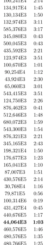
Tabel 2: Pareto-optimal solution without considering financial risk Variance Time
100,241E4 2:14 134,917E4 1:45 130,134E3 1:50 132,974E3 3:11 585,376E3 3:17 345,080E3 0:43 500,045E3 0:43 435,592E3 2:21 123,974E3 3:51 100,670E3 1:01 90,254E4 1:12 43,924E3 2:30 65,060E3 3:01 543,415E3 3:51 124,750E3 2:26 876,462E3 0:41 512,646E3 1:48 680,072E3 1:59 543,300E3 1:54 876,321E3 2:21 345,165E3 2:43 198,321E4 1:50 176,677E3 1:23 165,041E3 1:10 87,007E3 1:51 430,576E5 2:14 30,768E4 1:16 79,871E5 0:56 100,314E6 0:19 431,427E4 0:45 440,676E5 1:17
44,064E3 1:03
Based on the principle of Pareto-optimal solutions, according to the nu-merical results, it can be seen to have a high budget contained in the Pareto-optimal configurations from instance 32, which is the value of 2,300,000. Weightsg1 for the expected cost as low as 0.02. Weights for the purpose of
variance b2, very low at 0.231 with a low weight of g2 is 100. Then it can
be seen, the time of configuration has a small enough computing time, i.e during 1:03. Because in this solution dismissed the risk, then the value of the variance is minimized.
Then, performed comparison problem with considering the financial risk. In this case, the addition of weighting parameters for the weighting purpose of financial risk, i.e. b3 andg3. Thus, the formulation of
mathema-tical models have 11 binary variables, namely the number of configurations,
g1,g2,g3,b1,b2,b3, Ω, mean, variance, and time.
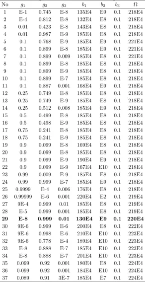
Table 3: Pareto-optimal solution with considering financial risk No g1 g2 g3 b1 b2 b3 Ω
1 E-1 0.745 E-8 135E4 E9 0.1 218E4 2 E-4 0.812 E-8 132E4 E8 0.1 218E4 3 0.01 0.423 E-8 143E4 E8 0.1 218E4 4 0.01 0.987 E-9 185E4 E8 0.1 218E4 5 0.1 0.768 E-9 185E4 E9 0.1 221E4 6 0.1 0.899 E-8 185E4 E9 0.1 221E4 7 0.1 0.899 0.009 185E4 E8 0.1 221E4 8 0.1 0.899 E-8 185E4 E8 0.1 218E4 9 0.1 0.899 E-9 185E4 E8 0.1 218E4 10 0.1 0.899 E-7 185E4 E8 0.1 218E4 11 0.1 0.887 0.001 168E4 E9 0.1 218E4 12 0.25 0.749 E-8 185E4 E8 0.1 218E4 13 0.25 0.749 E-9 185E4 E8 0.1 218E4 14 0.25 0.512 0.008 185E4 E9 0.1 218E4 15 0.5 0.499 E-8 185E4 E8 0.1 218E4 16 0.5 0.498 E-9 185E4 E8 0.1 218E4 17 0.75 0.241 E-8 185E4 E8 0.1 218E4 18 0.75 0.241 E-9 185E4 E8 0.1 218E4 19 0.9 0.099 E-8 169E4 E8 0.1 218E4 20 0.9 0.099 E-8 185E4 E8 0.1 218E4 21 0.9 0.099 E-9 190E4 E9 0.1 218E4 22 0.9 0.099 E-9 167E4 E10 0.1 218E4 23 0.99 0.009 E-9 185E4 E8 0.1 218E4 24 0.99 0.999 E-7 185E4 E9 0.1 218E4 25 0.9999 E-4 0.006 176E4 E8 0.1 218E4 26 0.99999 E-6 0.001 220E4 E2 0.1 219E4 27 9E-4 0.999 0.01 185E4 E8 0.1 219E4 28 E-5 0.999 0.001 185E4 E8 0.1 219E4
29 E-8 0.999 0.01 130E4 E9 0.1 220E4
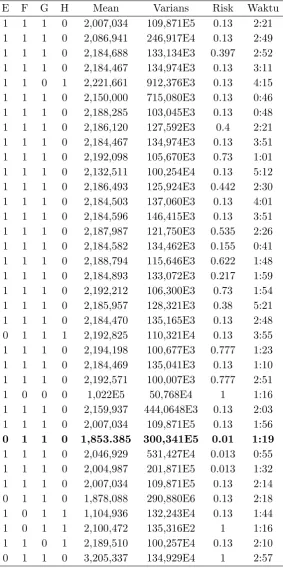
Tabel 3: Pareto-optimal solution with considering financial risk(continued)
E F G H Mean Varians Risk Waktu 1 1 1 0 2,007,034 109,871E5 0.13 2:21 1 1 1 0 2,086,941 246,917E4 0.13 2:49 1 1 1 0 2,184,688 133,134E3 0.397 2:52 1 1 1 0 2,184,467 134,974E3 0.13 3:11 1 1 0 1 2,221,661 912,376E3 0.13 4:15 1 1 1 0 2,150,000 715,080E3 0.13 0:46 1 1 1 0 2,188,285 103,045E3 0.13 0:48 1 1 1 0 2,186,120 127,592E3 0.4 2:21 1 1 1 0 2,184,467 134,974E3 0.13 3:51 1 1 1 0 2,192,098 105,670E3 0.73 1:01 1 1 1 0 2,132,511 100,254E4 0.13 5:12 1 1 1 0 2,186,493 125,924E3 0.442 2:30 1 1 1 0 2,184,503 137,060E3 0.13 4:01 1 1 1 0 2,184,596 146,415E3 0.13 3:51 1 1 1 0 2,187,987 121,750E3 0.535 2:26 1 1 1 0 2,184,582 134,462E3 0.155 0:41 1 1 1 0 2,188,794 115,646E3 0.622 1:48 1 1 1 0 2,184,893 133,072E3 0.217 1:59 1 1 1 0 2,192,212 106,300E3 0.73 1:54 1 1 1 0 2,185,957 128,321E3 0.38 5:21 1 1 1 0 2,184,470 135,165E3 0.13 2:48 0 1 1 1 2,192,825 110,321E4 0.13 3:55 1 1 1 0 2,194,198 100,677E3 0.777 1:23 1 1 1 0 2,184,469 135,041E3 0.13 1:10 1 1 1 0 2,192,571 100,007E3 0.777 2:51 1 0 0 0 1,022E5 50,768E4 1 1:16 1 1 1 0 2,159,937 444,0648E3 0.13 2:03 1 1 1 0 2,007,034 109,871E5 0.13 1:56
0 1 1 0 1,853.385 300,341E5 0.01 1:19
First set g in Table 3 Pareto-optimal configurations from instance 1 shows that the deviation of rupiah of the total expected cost of 1,350,000 is about 1,000,000 times as important to the total variance of the deviation unit cost of 1,000,000,000. Deviations from financial risks known by 0.1. In terms of Pareto-optimal configurations of from instance 1, the objective and the weight of the total expected costs and weights for financial risk is relatively low. According to the numerical results, the expected cost is the lowest of Pareto-optimal configuration from instance 29, with a value of 1,300,000. It has a relatively low risk which is equal to 0.01. Deviations from financial risk by 0.1. In the end, it is known that the computational time is also relatively small, i.e. for 1:19 but has a high variance of 300,000. Thus, from the results of numerical experiments of Table 2 and Table 3, the results of the comparison can be made to the table below:
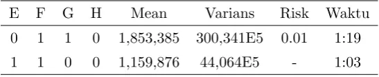
Table 4: The results of numerical comparisons No g1 g2 g3 b1 b2 b3 Ω
29 E-8 0.999 0.01 130E4 E9 0.1 220E4 32 0.02 0.231 - 125E4 E2 - 230E4
Tabel 4: The results of numerical comparisons(continued) E F G H Mean Varians Risk Waktu
0 1 1 0 1,853,385 300,341E5 0.01 1:19
1 1 0 0 1,159,876 44,064E5 - 1:03
5. CONCLUSION
After constraints, notation, and assumptions are described to develop a mathematical model formulation is sought, got Pareto-optimal solutions are obtained numerically from the formulation of goal achievement that is a variation of goal programming techniques. From the comparison of numer-ical experiments on samples of cases, the consideration of the financial risk involved in the model has a good effect due to the formation of the configu-ration of the optimal solution faster, i.e. the configuconfigu-ration from instance 29. Meanwhile, Pareto-optimal solution numerically without considering the fi-nancial risks contained in the configuration from instance 32. Therefore, a two-stage stochastic program approach with the concept of multi objective be a good way to capture the idea with high complexity of the supply chain design problems.
References
[1] Alborzi, F., Vafaei, M. H., Gholami, M. M., and Esfahani, S. (2011).A Multi-Objective Model for Supply Chain Network Design under Stochas-tic Demand. World Academy of Science, Engineering and Technology, Vol. 5, pp. 1776-1780.
[2] Azaron, A., Brown, K. N., Tarim, S. A., and Modarres, M. (2008). A multi-objective stochastic programming approach for supply chain de-sign considering risk. International Journal of Production Economics, Vol. 116, pp. 129-138.
[3] Barik, S. K., Biswal, M. P., and Chakravarty, D. (2012). Multiobjec-tive Two-Stage Stochastic Programming Problems with Interval Dis-crete Random Variables. Advances in Operation Research, Article ID 279181, pp. 1-21.
[4] Barbaro, A. F., and Bagajewicz, M. J. (2004). Managing financial risk in planning under uncertainty. International Journal of Production Eco-nomics, Vol. 50, pp. 963-989.
[5] Birge, J. R., and Louveaux, F. (1997). Introduction to Stochastic Pro-gramming. New York: Springer Verlag.
[6] Gregoriou, G. N., Hoppe, C., and Wehn, S. C. (2010). The Risk Mod-eling Evaluation Handbook. New York: McGraw-Hill Companies, Inc.
[8] Mirzapour, A. S. M. J., Baboli, A., Sadjadi, S. J., and Aryanezhad, M. B. (2011). A Multiobjective Stochastic Production-Distribution Plan-ning Problem in an Uncertain Environment Considering Risk and Workers Productivity. Mathematical Problems in Engineering, Article ID 406398, pp. 1-14.
[9] Uher, T. E and Toakley, A. R. (1999).Risk Management in the Concep-tual Phase of a Project. International Journal of Project Management, Vol. 3. pp. 161-169.
Siti Fatimah Sihotang: Graduate School of Mathematics, Faculty of Mathema-tics and Natural Sciences, University of Sumatera Utara, Medan 20155, Indonesia.
E-mail: [email protected]
Dame Meldaria Sipahutar : Graduate School of Mathematics, Faculty of Ma-thematics and Natural Sciences, University of Sumatera Utara, Medan 20155, In-donesia.
E-mail: [email protected]
Saib Suwilo: Department of Mathematics, Faculty of Mathematics and Natural Sciences, University of Sumatera Utara, Medan 20155, Indonesia.