Graph Clustering
and Minimum Cut Trees
Gary William Flake, Robert E. Tarjan, and Kostas Tsioutsiouliklis
Abstract.
In this paper, we introduce simple graph clustering methods based on minimum cuts within the graph. The clustering methods are general enough to apply to any kind of graph but are well suited for graphs where the link structure implies a notion of reference, similarity, or endorsement, such as web and citation graphs. We show that the quality of the produced clusters is bounded by strong minimum cut and expansion criteria. We also develop a framework for hierarchical clustering and present applications to real-world data. We conclude that the clustering algorithms satisfy strong theoretical criteria and perform well in practice.1. Introduction
Clustering data sets into disjoint groups is a problem arising in many domains. From a general point of view, the goal of clustering is to find groups that are both homogeneous and well separated, that is, entities within the same group should be similar and entities in different groups dissimilar. Often, data sets can be represented as weighted graphs, where nodes correspond to the entities to be clustered and edges correspond to a similarity measure between those entities.
The problem of graph clustering is well studied and the literature on the subject is very rich [Everitt 80, Jain and Dubes 88, Kannan et al. 00]. The best known graph clustering algorithms attempt to optimize specific criteria such as k-median, minimum sum, minimum diameter, etc. [Bern and Eppstein 96]. Other algorithms are application-specific and take advantage of the underlying structure or other known characteristics of the data. Examples are clustering © A K Peters, Ltd.
algorithms for images [Wu and Leahy 93] and program modules [Mancoridis et al. 98].
In this paper, we present a new clustering algorithm that is based on maximum
flow techniques, and in particular minimum cut trees. Maximumflow algorithms are relatively fast and simple, and have been used in the past for data-clustering (e.g., [Wu and Leahy 93], [Flake et al. 00]). The main idea behind maximumflow (or equivalently, minimum cut [Ford and Fulkerson 62]) clustering techniques, is to create clusters that have small intercluster cuts (i.e., between clusters) and relatively large intracluster cuts (i.e., within clusters). This guarantees strong connectedness within the clusters and is also a strong criterion for a good clus-tering, in general.
Our clustering algorithm is based on inserting an artificial sink into a graph that gets connected to all nodes in the network. Maximumflows are then calcu-lated between all nodes of the network and the artificial sink. A similar approach has been introduced in [Flake et al. 00], which was also the motivation for our work. In this paper we analyze the minimum cuts produced, calculate the quality of the clusters produced in terms of expansion-like criteria, generalize the cluster-ing algorithm into a hierarchical clustercluster-ing technique, and apply it to real-world data.
This paper consists of six sections. In Section 2, we review basic definitions necessary for the rest of the paper. In Section 3, we focus on the previous work of Flake et al. [Flake et al. 00], and then describe our cut-clustering algorithm and analyze it in terms of upper and lower bounds. In Section 4, we generalize the method of Section 3 by defining a hierarchical clustering method. In Section 5, we present results of our method applied to three real-world problem sets and see how the algorithm performs in practice. The paper ends with Section 6, which contains a summary of our results andfinal remarks.
2. Basic Definitions and Notation
2.1.
Minimum Cut Tree
Throughout this paper, we represent the web (or a subset of the web) as a directed graphG(V, E), with|V|=nvertices, and |E|=medges. Each vertex corresponds to a web page, and each directed edge to a hyperlink. The graph may be weighted, in which case we associate a real valued function w with an edge, and say, for example, that edge e = (u, v) has weight (or capacity)
Two subsetsAandBofV, such thatA∪B =V andA∩B=∅, define a cut in G, which we denote as (A, B). The sum of the weights of the edges crossing the cut defines its value. We use a real functioncto represent the value of a cut. So, cut (A, B) has valuec(A, B). In fact, functionccan also be applied whenA
andB do not coverV, butA∪B ⊂V.
Our algorithms are based on minimum cut trees, which were defined in [Go-mory and Hu 61]. For graph G, there exists a weighted graph TG, which we
call the minimum cut tree (or simply, min-cut tree) of G. The min-cut tree is defined overV and has the property that we canfind the minimum cut between two nodes s, t in G by inspecting the path that connectss and t in TG. The
edge of minimum capacity on that path corresponds to the minimum cut. The capacity of the edge is equal to the minimum cut value, and its removal yields two sets of nodes inTG, but also inG, which correspond to the two sides of the
cut. For every undirected graph, there always exists a min-cut tree. Gomory and Hu [Gomory and Hu 61] describe min-cut trees in more detail and provide an algorithm for calculating min-cut trees.
2.2.
Expansion and Conductance
In this subsection, we discuss a small number of clustering criteria and compare and contrast them to one another. We initially focus on two related measures of intracluster quality and then briefly relate these measures to intercluster quality. Let (S,S¯) be a cut inG. We define the expansion of a cut as [Kannan et al. 00]:
ψ(S) =
u∈S,v∈S¯w(u, v) min{|S|,|S¯|} ,
where w(u, v) is the weight of edge (u, v). The expansion of a (sub)graph is the minimum expansion over all the cuts of the (sub)graph. The quality of a clustering can be measured in terms of expansion: the expansion of a clustering of G is the minimum expansion over all its clusters. The larger the expansion of the clustering, the higher its quality. One way to think about the expansion of a clustering is that it serves as a strict lower bound for the expansion of any intracluster cut for a graph.
We can also define conductance, which is similar to expansion except that it weights cuts inversely by a function of edge weight instead of the number of vertices in a cut set. For the cut (S,S¯) inG, conductance is defined as [Kannan et al. 00]:
φ(S) =
where c(S) = c(S, V) = u∈Sv∈V w(u, v). As with expansion, the conduc-tance of a graph is the minimum conducconduc-tance over all the cuts of the graph. For a clustering of G, let C ⊆ V be a cluster and (S, C−S) a cluster within C, whereS⊆C. The conductance ofS inC is [Kannan et al. 00]:
φ(S, C) =
u∈S,v∈C−Sw(u, v)
min{c(S), c(C−S)}.
The conductance of a clusterφ(C) is the smallest conductance of a cut within the cluster; for a clustering the conductance is the minimum conductance of its clusters. Thus, the conductance of a clustering acts as a strict lower bound on the conductance of any intracluster cut.
Both expansion and conductance seem to give very good measures of quality for clusterings and are claimed in [Kannan et al. 00] to be generally better than simple minimum cuts. The main difference between expansion and conductance is that expansion treats all nodes as equally important while conductance gives greater importance to nodes with high degree and adjacent edge weight.
However, both expansion and conductance are insufficient by themselves as clustering criteria because neither enforces qualities pertaining to intercluster weight, nor the relative size of clusters. Moreover, there are difficulties in directly optimizing either expansion or conductance because both are computationally hard to calculate, usually raising problems that are NP-hard, since they each have an immediate relation to thesparsest cutproblem. Hence, approximations must be employed.
With respect to the issue of simultaneously optimizing both intra- and inter-cluster criteria, Kannan et al. [Kannan et al. 00] have proposed a bicriteria optimization problem that requires:
1. clusters must have some minimum conductance (or expansion)α, and 2. the sum of the edge weights between clusters must not exceed some
maxi-mum fraction of the sum of the weights of all edges inG.
The algorithm that we are going to present has a similar bicriterion. It provides a lower bound on the expansion of the produced clusters and an upper bound on the edge weights between each cluster and the rest of the graph.
3. Cut-Clustering Algorithm
3.1.
Background and Related Work
minimum cut trees. Whileflows and cuts are well defined for both directed and undirected graphs, minimum cut trees are defined only for undirected graphs. Therefore, we restrict, for now, the domain to undirected graphs. In Section 5, we will address the issue of edge direction and how we deal with it.
LetG(V, E) be an undirected graph, and lets, t∈V be two nodes ofG. Let (S, T) be the minimum cut between sandt, where s∈S andt∈T. We define
S to be thecommunityofsinGwith respect tot. If the minimum cut between
sandtis not unique, we choose the minimum cut that minimizes the size ofS. In that case, it can be shown thatS is unique [Gomory and Hu 61].
The work presented in this paper was motivated by the paper of Flake et al. [Flake et al. 00]. There, aweb communityis defined in terms of connectivity. In particular, a web community S is defined as a collection of nodes that has the property that all nodes of the web community predominantly link to other web community nodes. That is,
3
v∈S
w(u, v)>3
v∈S¯
w(u, v),∀u∈S. (3.1)
We briefly establish a connection between our definition of a community and web communities from [Flake et al. 00]. The following lemma applies:
Lemma 3.1.
For an undirected graph G(V, E), let S be a community of s with respect to t. Then,3
v∈S
w(u, v)>3
v∈S¯
w(u, v),∀u∈S−{s}. (3.2)
Proof.
Since S is a community of s with respect to t, the cut (S, V −S) is a minimum cut for s and t in G. Thus, every node w∈ S−{s} has more edge weight to the nodes ofSthan to the nodes ofV−S; otherwise, movingwto the other side of the cut (S, T) would yield a smaller cut betweensandt.Lemma 3.1 shows that a communityS based on minimum cuts is also a web community. The only node to possibly violate the web community property is the sourcesitself. In that case, it is usually a good indication that the community ofsshould actually be a larger community that containsS as a subset. At this point we should also point out the inherent difficulty offinding web communities with the following theorem:
Proof.
The proof is given in Section 7. (Note thatkcan be at mostn/2, since no single node can form a community by itself. Also, k >1, since fork= 1, the set of all nodes forms a trivial community.)3.2.
Cut-Clustering Algorithm
At this point we extend the definition of a communitySofs, when notis given. To do this, we introduce an artificial nodet, which we call theartificial sink. The artificial sink is connected to all nodes ofGvia an undirected edge of capacityα. We can now consider the community S ofsas defined before, but with respect to the artificial sink,t. We can now show our main theorem:
Theorem 3.3.
Let G(V, E) be an undirected graph, s∈V a source, and connect an artificial sink t with edges of capacity α to all nodes. Let S be the community of s with respect to t. For any nonempty P andQ, such that P ∪Q=S andP∩Q=∅, the following bounds always hold:
c(S, V −S)
|V −S| ≤α≤
c(P, Q)
min(|P|,|Q|). (3.3)
Theorem 3.3 shows that α serves as an upper bound of the intercommunity edge capacity and a lower bound of the intracommunity edge capacity. In Sec-tion 2.2, we saw that the expansion for a subsetSofV is defined as the minimum value ofφ(S) = min(|c(P,QP|,|)Q|), for all cuts (P, Q) of S. Thus, a community of G
with respect to the artificial sink will have expansion at least α. The left side of inequality (3.3) bounds the intercommunity edge capacity, thus guaranteeing that communities will be relatively disconnected. Thus,αcan be used to control the trade-offbetween the two criteria. We will discuss the choice of αand how it affects the community more extensively in Section 3.3.
To prove Theorem 3.3 we prove a series of lemmata. Butfirst we defineGαto be theexpanded graphofG, after the artificial sinktis connected to all nodesV
with weightα.
Lemma 3.4.
Let s, t∈V be two nodes ofG and letS be the community of s with respect tot. Then, there exists a min-cut treeTG ofG, and an edge(a, b)∈TG, such that the removal of(a, b)yields S andV −S.Note that the issue raised in this lemma is that there may be multiple min-cut trees forG. Despite this fact, there always exists at least one min-cut treeTG,
Proof.
Gomory and Hu prove the existence of a min-cut tree for any undirected graph Gby construction. Their proof starts offwith an arbitrary pair of nodesa, b, finds a minimum cut (A, B) betweena andb, and constructs the min-cut tree recursively. The resulting min-cut tree contains (a, b) as an edge. To prove the lemma, it suffices to picka=s, b=t, and the minimum cut (S, V −S) as starting points.
Lemma 3.5.
LetTG be a min-cut tree of a graphG(V, E), and let(u, w)be an edge of TG. Edge(u, w) yields the cut(U, W) inG, withu∈U,w∈W. Now, take any cut (U1, U2)of U, so that U1 and U2 are nonempty, u∈U1, U1∪U2=U, andU1∩U2=∅. Then,c(W, U2)≤c(U1, U2). (3.4)
Note that this lemma defines a type of triangle inequality for flows and cuts that will be frequently used in the proofs that follow.
Proof.
Since (u, w) is an edge ofTG, it defines a minimum cut (U, W) betweenuandwin G. Now consider the cut (U1, W∪U2). Since u∈U1 andw∈W, the cut (U1, W∪U2) is also a cut betweenuand w, but not necessarily minimum. Hence, we can write
c(U, W)≤c(U1, W∪U2), (3.5)
c(U1∪U2, W)≤c(U1, W∪U2), (3.6)
c(U1, W) +c(U2, W)≤c(U1, W) +c(U1, U2), (3.7)
c(U2, W)≤c(U1, U2). (3.8)
Lemma 3.6.
Let Gα be the expanded graph of G, and let S be the community ofs with respect to the artificial sink t. For any nonempty P and Q, such that
P∪Q=S andP∩Q=∅, the following bound always holds:
α≤ c(P, Q)
min(|P|,|Q|). (3.9)
Proof.
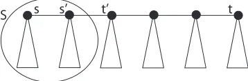
LetTGα be a minimum cut tree ofGα, and let (s , t) be an edge of TGαwhose removal yieldsS andV−S∪{t}inGα. According to Lemma 3.4, such a
TGα exists, and by the definition of a min-cut tree, (s , t) lies on the path from
Figure 1. Min-cut treeTGα with emphasis on the (s,t)-path. Triangles correspond
to subtrees that are not part of the path.
Now, we split S into two subsets P andQ, and assume w.l.o.g. thats ∈P. Then, Lemma 3.5 applies and yields
c(V −S∪{t}, Q) ≤ c(P, Q), (3.10)
c(V −S, Q) +c({t}, Q) ≤ c(P, Q), (3.11)
c({t}, Q) ≤ c(P, Q), (3.12)
α|Q| ≤ c(P, Q), (3.13)
α·min(|P|,|Q|) ≤ c(P, Q). (3.14) Inequality (3.13) is true becausetis connected to every node inV with an edge of weightα, and inequality (3.14) implies the lemma.
Lemma 3.7.
Let Gα be the expanded graph ofG(V, E)and letS be the community of swith respect to the artificial sinkt. Then, the following bound always holds:c(S, V −S)
|V −S| ≤α. (3.15)
Proof.
As in the previous lemma, let TGα be a minimum cut tree of Gα thatcontains an edge (s , t), the removal of which yields setsS andV −S∪{t}. By the definition of a min-cut tree, (s , t) corresponds to a minimum cut between
s andt inGα. The value of this minimum cut is equal toc(S, V −S∪{t}). Now, consider the cut (V,{t}) in Gα. It also separates s from t, but is not necessarily a minimum cut between them. This means
c(S, V −S∪{t}) ≤ c(V,{t}), (3.16)
c(S, V −S) +c(S,{t}) ≤ c(V −S,{t}) +c(S,{t}), (3.17)
c(S, V −S) ≤ c(V −S,{t}), (3.18)
c(S, V −S) ≤ α|V −S|. (3.19)
Now we can prove Theorem 3.3.
Proof.
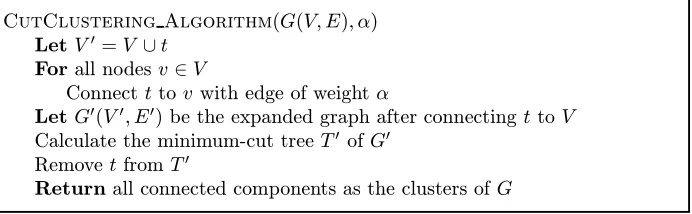
Immediate by combination of Lemmata 3.6 and 3.7.We can use the above ideas to eitherfind high-quality communities inG, or to develop a general clustering algorithm based on the min-cut tree ofG. Figure 2 shows the cut-clustering algorithm. The idea is to expand G to Gα, find the min-cut tree TGα, remove the artificial sink t from the min-cut tree, and the
resulting connected components form the clusters ofG. CutClustering Algorithm(G(V, E),α)
LetV =V ∪t Forall nodesv∈V
Connectt tov with edge of weightα
LetG(V , E) be the expanded graph after connecting ttoV
Calculate the minimum-cut treeT ofG
Removetfrom T
Returnall connected components as the clusters of G
Figure 2. Cut-clustering algorithm.
So, Theorem 3.3 applies to all clusters produced by the cut-clustering algo-rithm, giving lower bounds on their expansion and upper bounds on the inter-cluster connectivity.
3.3.
Choosing
αWe have seen that the value ofαin the expanded graphGαplays a crucial role in the quality of the produced clusters. But how does it relate to the number and sizes of clusters, and what is a good choice forα?
It is easy to see that asαgoes to 0, the min-cut betweentand any other node
vofGwill be the trivial cut ({t}, V), which isolatestfrom the rest of the nodes. So, the cut-clustering algorithm will produce only one cluster, namely the entire graphG, as long asGis connected. On the other extreme, asαgoes to infinity it will cause TGα to become a star with the artificial sink at its center. Thus,
the clustering algorithm will producentrivial clusters, all singletons.
The nesting property of min-cuts has been used by Gallo et al. [Gallo et al. 89] in the context of parametric maximumflow algorithms. A parametric graph is defined as a regular graphGwith sourcesand sinkt, with edge weights being linear functions of a parameterλ, as follows:
1. wλ(s, v) is a nondecreasing function ofλfor allv=t. 2. wλ(v, t) is a nonincreasing function ofλfor allv=s. 3. wλ(v, w) is constant for allv=s,w=t.
A maximum flow (or minimum cut) in the parametric graph G corresponds to a maximumflow (or minimum cut) inGfor some particular value ofλ. One can immediately see that the parametric graph is a generalized version of our expanded graph Gα, since the edges adjacent to the artificial sink are a linear function of α, and no other edges in Gα are parametric. We can use both nondecreasing and nonincreasing values for α, since t can be treated as either the sink or the source inGα.
The following nesting property lemma holds forGα:
Lemma 3.8.
For a sourcesinGαi, whereαi∈{α1, ...,αmax}, such thatα1<α2<... < αmax, the communities S1, ..., Smax are such that S1 ⊆S2 ⊆... ⊆ Smax, whereSi is the community ofswith respect tot inGai.
Proof.
This is a direct result of a similar lemma in [Gallo et al. 89].In fact, in [Gallo et al. 89] it has been shown that for a given s the total number of different communities Si is no more than n−2 regardless of the
number of ai and they can all be computed in time proportional to a single
max-flow computation, by using a variation of the Goldberg-Tarjan preflow-push algorithm [Goldberg and Tarjan 88].
Thus, if we want tofind a cluster ofsinGof certain size or other characteristic we can simply use this methodology,find all clusters fast, and then choose the best clustering according to a metric of our choice. Also, because the parametric preflow algorithm in [Gallo et al. 89] finds all clusters either in increasing or decreasing order, we can stop the algorithm as soon as a desired cluster has been found. We will use the nesting property again, in Section 4, when describing the hierarchical cut-clustering algorithm.
3.4.
Heuristic for the Cut-Clustering Algorithm
undert. But calculating the min-cut tree can be equivalent to computingn−1 maximum flows [Gomory and Hu 61], in the worst case. Therefore, we use a heuristic that, in practice, finds the clusters of Gmuch faster, usually in time proportional to the total number of clusters.
Lemma 3.9.
Let v1, v2 ∈ V, and S1, S2 be their communities with respect to t inGα. Then eitherS1 andS2 are disjoint or one is a subset of the other.
Proof.
This is a special case of a more general lemma in [Gomory and Hu 61]. If S1 and S2 overlap without one containing the other, then either S1∩S2 orS1−S2is a smaller community forv1, or symmetrically, eitherS1∩S2orS2−S1 is a smaller community forv2. ThusS1andS2 are disjoint or one is a subset of the other.
A closer look at the cut-clustering algorithm shows that it suffices to find the minimum cuts that correspond to edges adjacent to t in TGα. So, instead of
calculating the entire min-cut tree ofGα, we use Lemma 3.9 in order to reduce the number of minimum cut computations necessary. If the cut between some nodevandtyields the communityS, then we do not use any of the nodes inSas subsequent sources tofind minimum cuts witht, since according to the previous lemma they cannot produce larger communities. Instead, we mark them as being in communityS, and later ifSbecomes part of a larger community S we mark all nodes ofS as being part ofS. Obviously, the cut-clustering algorithmfinds the largest communities betweentand all nodes inV.
The heuristic relies on the choice of the next node for which wefind its mini-mum cut with respect tot. The larger the next cluster, the smaller the number of minimum cut calculations. Prior to any min-cut calculations, we sort all nodes according to the sum of the weights of their adjacent edges, in decreasing order. Each time, we compute the minimum cut between the next unmarked node andt. We have seen, in practice, that this reduces the number of max-flow computations almost to the number of clusters inG, speeding up the algorithm significantly.
4. Hierarchical Cut-Clustering Algorithm
possible loops get deleted and parallel edges are combined into a single edge with weight equal to the sum of their weights.
When applying the cut-clustering algorithm on the contracted graph, we sim-ply choose a new α-value, and the new clustering, now, corresponds to a clus-tering of the clusters of G. By repeating the same process a number of times, we can build a hierarchy of clusters. Notice that the newαhas to be of smaller value than the last, for otherwise the new clustering will be the same, since all contracted nodes will form singleton clusters.
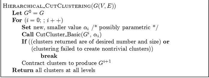
The quality of the clusters at each level of the hierarchy is the same as for the initial basic algorithm, depending each time on the value of α, however the expansion measure is now over the clusters instead of over the nodes. The iterative cut-clustering algorithm stops either when the clusters are of a desired number and/or size, or when only a single cluster that contains all nodes is identified. The hierarchical cut-clustering algorithm is described in Figure 3.
Hierarchical CutClustering(G(V, E))
LetG0=G For(i= 0; ;i+ +)
Set new, smaller valueαi /* possibly parametric */ Call CutCluster Basic(Gi,α
i)
If((clusters returned are of desired number and size)or
(clustering failed to create nontrivial clusters))
break
Contract clusters to produceGi+1
Returnall clusters at all levels
Figure 3. Hierarchical cut-clustering algorithm.
The hierarchical cut-clustering algorithm provides a means of looking at graph
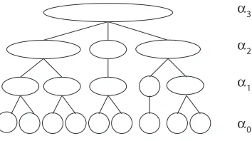
G in a more structured, multilevel way. We have used this algorithm in our experiments to find clusters at different levels of locality. Figure 4 shows what a hierarchical tree of clusters looks like. At the lower levels α is large and the clusters are small and dense. At higher levels, the clusters are larger in size and sparser. Also notice that the clusters at higher levels are always supersets of clusters at lower levels. This is expressed in the following lemma, the proof of which follows directly from the nesting property.
Lemma 4.1.
Let α1 > α2 > ... > αmax be a sequence of parameter values that connect t to V in Gai. Let αmax+1 ≤αmax be small enough to yield a singleFigure 4. Hierarchical tree of clusters.
produced by eachαi, and all clusterings together form a hierarchical tree over the clusterings of G.
5. Experimental Results
5.1.
CiteSeer
CiteSeer [CiteSeer 97] is a digital library for scientific literature. Scientific liter-ature can be viewed as a graph, where the documents correspond to the nodes and the citations between documents to the edges that connect them. The cut-clustering algorithms require the graph to be undirected, but citations, like hyperlinks, are directed. In order to transform the directed graph into undi-rected, we normalize over all outbound edges for each node (so that the total sums to unity), remove edge-directions, and combine parallel edges. Parallel edges resulting from two directed edges are resolved by summing the combined weight.
Our normalization is similar to the first iteration of HITS [Kleinberg 98] and to PageRank [Brin and Page 98] in that each node distributes a constant amount of weight over its outbound edges. The fewer pages to which a node points, the more influence it can pass to the neighbors to whom it points.
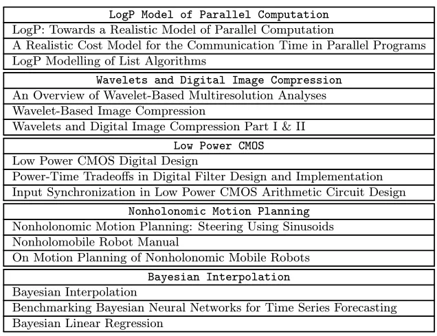
By looking at the resulting clusters, we concluded that at lower levels the clusters contain nodes that correspond to documents with very specific content. For example, there are small clusters (usually with fewer than ten nodes) that focus on topics like “LogP Model of Parallel Computation,” “Wavelets and Dig-ital Image Compression,” “Low Power CMOS,” “Nonholonomic Motion Plan-ning,” “Bayesian Interpolation,” and thousands of others. Table 1 shows the titles of three documents of each of the clusters just mentioned. For each clus-ter, these three documents are, respectively, the heaviest, median, and lightest linked within their clusters. We can see that the documents are closely related to each other. This was the case in all clusters of the lowest level.
LogP Model of Parallel Computation LogP: Towards a Realistic Model of Parallel Computation
A Realistic Cost Model for the Communication Time in Parallel Programs LogP Modelling of List Algorithms
Wavelets and Digital Image Compression An Overview of Wavelet-Based Multiresolution Analyses Wavelet-Based Image Compression
Wavelets and Digital Image Compression Part I & II Low Power CMOS Low Power CMOS Digital Design
Power-Time Tradeoffs in Digital Filter Design and Implementation Input Synchronization in Low Power CMOS Arithmetic Circuit Design
Nonholonomic Motion Planning Nonholonomic Motion Planning: Steering Using Sinusoids Nonholomobile Robot Manual
On Motion Planning of Nonholonomic Mobile Robots Bayesian Interpolation Bayesian Interpolation
Benchmarking Bayesian Neural Networks for Time Series Forecasting Bayesian Linear Regression
Table 1. CiteSeer data–example titles are from the highest, median, and lowest ranking papers within a community, thus demonstrating that the communities are topically focused.
For clusters of higher levels, we notice that they combine clusters of lower levels and singletons that have not yet been clustered with other nodes. The clusters of these levels (after approximately ten iterations) focus on more general topics, like “Concurrent Neural Networks,” “Software Engineering, Verification, Validation,” “DNA and Bio Computing,” “Encryption,” etc.
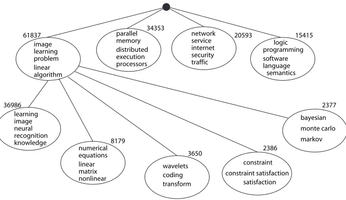
Lan-algorithm
Figure 5. Top-level clusters of CiteSeer. The sizes of each cluster are shown, as well as the top features for each cluster.
guages.” Figure 5 shows the highest nontrivial level, consisting of four clusters. In order to better validate our results, for each cluster, we have extracted text features (i.e., uni-grams and bi-grams) from the title and abstract of the papers. For each feature we calculated the expected entropy loss of the feature charac-terizing the pages within a cluster, relative to the pages outside that cluster.
Figure 5 shows thefive highest ranking features for each cluster. Also, the sizes
of the clusters are shown, as well as the second level for the largest cluster. Based on the features, we can see that the four major clusters in CiteSeer are: “Algo-rithms and Graphics,” “Systems,” “Networks and Security,” and “Software and Programming Languages.”
As can be seen, the iterative cut-clustering algorithm yields a high-quality clustering, both on the large scale and small scale, as supported by the split of topics on the top level, and the focused topicality on the lowest level clusters.
Also, because of the strict bounds that the algorithm imposes on the expansion
for each cluster, it may happen that only a subgraph of G gets clustered into
5.2.
Open Directory
The Open Directory Project [Dmoz 98], or dmoz, is a human-edited directory of the web. For our experiment we start off with the homepage of the Open Directory, http://www.dmoz.org, and crawl all web pages up to two links away, in a breadth-first approach. This produces 1,624,772 web pages. The goal is to see if and how much the clusters produced by our cut-clustering algorithm coincide with those of the human editors.
In order to cluster these web pages, we represent them as nodes of a graph, where the edges correspond to hyperlinks between them, but we exclude all links between web pages of the same domain, because this biases the graph. We also exclude any internal dmoz links. We will elaborate more on how internal links affect the clustering at the end of this section. The final graph is disconnected, with the largest connected component containing 638,458 nodes and 845,429 edges. The cut-clustering algorithm can be applied to each connected component separately, or to the entire graph at once. For reasons of simplicity, and since the graph is not too large to handle, we choose the second approach. The average node degree of the graph is 1.47. Similar to the CiteSeer data, before applying the clustering algorithm, we make the graph undirected and normalize the edges over the outbound links.
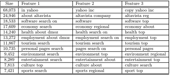
Applying the cut-clustering algorithm for various values of α, we build the hierarchical tree of Figure 4 for this graph. Naturally, at the highest level we get the connected components of the initial graph. For the next two levels, only small pieces of the connected components are being cut off. At level four, the largest connected component gets broken up into hundreds of smaller clusters. There are many clusters that contain a few hundred nodes. The largest cluster contains about 68,073 nodes. Table 2 shows the 12 largest dmoz clusters and the top three features extracted for each of them. We notice that the top two clusters contain web pages that refer to or are from the search engines Yahoo! and Altavista, reflecting their popularity and large presence in the dmoz category. The other ten clusters correspond to categories at the highest or second highest level of dmoz. In fact, 88 of the top 100 clusters correspond to categories of dmoz at the two highest levels. Regarding the coverage of the clusters, the top 250 clusters cover 65 percent of the total number of nodes, and the top 500 clusters cover over 85 percent.
Compared to the CiteSeer data, we conclude that the dmoz clusters are rel-atively smaller, but more concentrated. This is most likely the result of the extremely sparse dmoz graph. Still, the cut-clustering algorithm is able to ex-tract the most important categories of dmoz. A limitation of our algorithm is in
Size Feature 1 Feature 2 Feature 3
68,073 in yahoo yahoo inc copy yahoo inc
24,946 about altavista altavista company altavista reg 18,533 software search on software software top 17,609 economy search economy regional economy about 14,240 health about dmoz health search on health top 13,272 employment about dmoz employment search on employment top 11,867 tourism search tourism search tourism top 10,735 personal pages search pages search on personal pages
9,452 environment search environment top environment regional 8,289 entertainment search entertainment about entertainment top 7,813 culture top culture about culture search 7,421 sports search sports regional sport top
Table 2. Top three features for largest dmoz clusters.
of dmoz, but this is also a result of the sparseness of the graph. We have applied less restrictive clustering algorithms on top of the cut-clustering algorithm, such as agglomerate and k-means algorithms, and were able to add an intermediate level to the hierarchical tree that almost coincided with the top-level categories of dmoz.
Regarding internal links, if we repeat the same experiment without excluding any internal links within dmoz or between two web pages of the same site, the results are not as good. Internal links force clusters to be concentrated more around individual web sites. In particular, when a web site has many internal links, because of normalization, the external links get less weight and the results are skewed toward isolating the web site. We suggest that internal and external links should be treated independently. In our examples we ignored internal links entirely, but one could also assign some small weight to them by normalizing internal and external links separately, for example.
5.3.
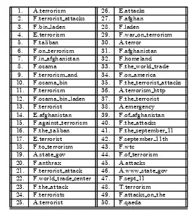
The 9/11 Community
1. A.terrorism 26. E.attacks 2. F.terrorist attacks 27. F.afghan 3. F.bin laden 28. F.laden
4. E.terrorism 29. F.war on terrorism 5. F.taliban 30. A.terror
6. F.on terrorism 31. F.afghanistan 7. F.in afghanistan 32. F.homeland 8. F.osama 33. F.the world trade 9. F.terrorism and 34. F.on america
10. F.osama bin 35. F.the terrorist attacks 11. F.terrorism 36. A.terrorism http 12. F.osama bin laden 37. F.the terrorist 13. F.terrorist 38. A.emergency 14. E.afghanistan 39. F.of afghanistan 15. F.against terrorism 40. F.the attacks 16. F.the taliban 41. F.the september 11 17. E.terrorist 42. F.september 11th 18. F.to terrorism 43. F.wtc
19. A.state gov 44. F.of terrorism 20. F.anthrax 45. A.attacks 21. F.terrorist attack 46. A.www state gov 22. F.world trade center 47. F.sept 11 23. F.the attack 48. T.terrorism 24. F.terrorists 49. F.attacks on the 25. A.terrorist 50. F.qaeda
Table 3. Top 50 features of the 9/11 community. A prefix A, E, or F indicates whether the feature occurred in the anchor text, extended anchor text (that is, anchor text including some of the surrounding text), or full text of the page, respectively.
only the link structure of the web graph, all top features, as extracted from the text, show the high topical concentration of the 9/11 community.
6. Conclusions
While identifying communities is an NP-complete problem (see Section 7 for more details), we partially resolve the intractability of the underlying problem by limiting what communities can be identified. More specifically, the cut-clustering algorithm identifies communities that satisfy the strict bicriterion imposed by the choice ofα, and no more. The algorithm is not even guaranteed tofind all communities that obey the bounds, just those that happen to be obvious in the sense that they are visible within the cut tree of the expanded graph. Hence, the main strength of the cut-clustering algorithm is also its main weakness: it avoids computational intractability by focusing on the strict requirements that yield high-quality clusterings.
All described variations of the cut-clustering algorithm are relatively fast (es-pecially with the use of the heuristic of Section 3.4), simple to implement, and give robust results. Theflexibility of choosingα, and thus determining the qual-ity of the clusters produced, is another advantage. Additionally, whenαis not supplied, we canfind all breakpoints ofαfast [Gallo et al. 89].
On the other hand, our algorithms are limited in that they do not parameterize over the number and sizes of the clusters. The clusters are a natural result of the algorithm and cannot be set as desired (unless searched for by repeated calculations). Also note that cut clusters are not allowed to overlap, which is problematic for domains in which it seems more natural to assign a node to multiple categories (something we have also noticed with the CiteSeer data set). This issue is a more general limitation of all clustering algorithms that produce hard or disjoint clusters.
Implementation-wise, maximum flow algorithms have significantly improved in speed over the past years ([Goldberg 98], [Chekuri et al. 97]), but they are still computationally intense on large graphs, being polynomial in complexity. Randomized or approximation algorithms could yield similar results, but in less time, thus laying the basis for very fast cut-clustering techniques of high quality.
7. Proof of Theorem 3.2
We now provide a proof of Theorem 3.2 in Section 3. In fact, we shall prove a slightly more general theorem:
PROBLEM:PARTITION INTO COMMUNITIES INSTANCE: Undirected, weighted graphG(V, E), real parameterp≥1/2, integer k.
QUESTION: Can the vertices ofGbe partitioned into kdisjoint sets
V1, V2, ..., Vk, such that for1≤i≤k, the subgraph ofGinduced by Vi is a PARTITION INTO COMMUNITIES isN P-complete.
Proof.
We will prove the above theorem by reducing BALANCED PARTITION, a restricted version of PARTITION, to PARTITION INTO COMMUNITIES.Here are the definitions of PARTITION (from [Garey and Johnson 79]) and BALANCED PARTITION.
PROBLEM:PARTITION
INSTANCE: Afinite setAand a sizes(a)∈Z+ for each a∈A. QUESTION: Is there a subsetA ⊆Asuch that
QUESTION: Is there a subsetA ⊆A
such thata∈AIs(a) =
a∈A−AIs(a), and|A|=|A|/2?
Both PARTITION and BALANCED PARTITION are well-known NP-complete problems ([Karp 72] and [Garey and Johnson 79]). To prove Theorem 7.1 we will reduce BALANCED PARTITION to COMMUNITIES.
First, it is easy to see that a given solution for COMMUNITIES is verifiable in polynomial time, by checking whether each node is connected to nodes of the same cluster by at least a fractionpof its total adjacent edge weight.
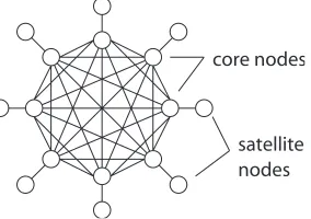
We transform the input to BALANCED PARTITION to that of COMMU-NITIES. The input set C has cardinality n= 2k. We construct an undirected graph G with 2n+ 4 nodes as follows. First, n of G’s nodes form a complete graphKnwith all edge weights equal tow, where s(aminn ) > w >0, andaminhas
the smallest sizes(amin) among all elementsai ofA. Let us call these nodes the core nodesof the graph. Next, a satellite node is connected to each core node, with edge weight w+ , such that min{w
2,
|s(ai)−s(aj)|
n } > >0, for allai and
Figure 6. Core and satellite nodes forming the core graph.
Now, we add two more nodes to the graph, which we callbase nodes. Every core node is connected to both base nodes by edges of equal weight. We make sure that each core node is connected to the base nodes by a differents(ai) value.
Finally, we add two more satellite nodes, one to each base node, with edges of weight . See Figure 7 for thefinal graph.
Figure 7. Final graph with base nodes.
Now, let us assume that COMMUNITIES is solvable in polynomial time. We transform an input of BALANCED PARTITION as mentioned above, and set
p= 1/2 andk= 2.
Assume that COMMUNITIES gives a solution for this instance. Then, the following statements can be verified (we leave the proofs to the reader):
1. the solution must partition the core nodes into two nonempty sets, sayS1 andS2.
4. all satellite and core nodes satisfy the community property, that is, they are more strongly connected to other community members than to non-members.
Notice that the last statement does not include base nodes. Is it possible that their adjacent weight is less within their community? The answer depends on how the core nodes get divided. If the core nodes are divided in such a way that the sum of their adjacent ai values is equal for both sets, then it is
easy to verify that the base nodes do not violate the community property. In the opposite case, one of the two base nodes will be more strongly connected to the nodes of the other community than to the nodes of its own community. Thus, the only possible solution for COMMUNITIES must partition all ai into
two sets of equal sum and cardinality. But this implies that any instance to the BALANCED PARTITION problem can be solved by COMMUNITIES. And since BALANCED PARTITION isN P-complete and we can build the graphG
and transform the one instance to the other in polynomial time, PARTITION INTO COMMUNITIES is NP-complete, as well.
References
[Bern and Eppstein 96] M. Bern and D. Eppstein. “Approximation Algorithms for Geometric Problems.” In Approximation Algorithms for NP-Hard Problems, edited by D. S. Hochbaum, pp. 296—345. Boston: PWS Publishing Company, 1996.
[Brin and Page 98] S. Brin and L. Page. “Anatomy of a Large-Scale Hypertextual Web Search Engine.” In Proc. 7th International World Wide Web Conference, pp. 107—117. New York: ACM Press, 1998.
[Chekuri et al. 97] C. S. Chekuri, A. V. Goldberg, D. R. Karger, M. S. Levine, and C. Stein. “Experimental Study of Minimum Cut Algorithms.” In Proc. 8th ACM-SIAM Symposium on Discrete Algorithms, pp. 324—333. Philadelphia: SIAM Press, 1997.
[Cherkassky and Goldberg 97] B. V. Cherkassky and A. V. Goldberg. “On Imple-menting Push-Relabel Method for the Maximum Flow Problem.” Algorithmica 19 (1997), 390—410.
[CiteSeer 97] CiteSeer. Available from World Wide Web (http://www.citeseer.com), 1997.
[Dmoz 98] Dmoz. Available from World Wide Web (http://www.dmoz.org), 1998.
[Flake et al. 00] G. W. Flake, S. Lawrence, and C. L. Giles. “Efficient Identification of Web Communities.” InProceedings of the Sixth International Conference on Knowledge Discovery and Data Mining (ACM SIGKDD-2000), pp. 150—160. New York: ACM Press, 2000.
[Ford and Fulkerson 62] L. R. Ford Jr. and D. R. Fulkerson.Flows in Networks. Prince-ton: Princeton University Press, 1962.
[Gallo et al. 89] G. Gallo, M. D. Grigoriadis, and R. E. Tarjan. “A Fast Parametric Maximum Flow Algorithm and Applications.” SIAM Journal of Computing18:1 (1989), 30—55.
[Garey and Johnson 79] M. R. Garey and D. S. Johnson.Computers and Intractability: A Guide to the Theory of NP-Completeness. New York: Freeman, 1979.
[Goldberg 98] A. V. Goldberg. “Recent Developments in Maximum Flow Algorithms.” Technical Report No. 98-045, NEC Research Institute, Inc., 1998.
[Goldberg and Tarjan 88] A. V. Goldberg and R. E. Tarjan. “A New Approach to the Maximum Flow Problem.” J. Assoc. Comput. Mach.35 (1998), 921—940.
[Goldberg and Tsioutsiouliklis] A. V. Goldberg and K. Tsioutsiouliklis. “Cut Tree Algorthms: An Experimental Study.” J. Algorithms.38:1 (2001), 51—83.
[Gomory and Hu 61] R. E. Gomory and T. C. Hu. “Multi-Terminal Network Flows.” J. SIAM9 (1961), 551—570.
[Hu 82] T. C. Hu. Combinatorial Algorithms. Reading, MA: Addison-Wesley, 1982.
[Jain and Dubes 88] A. K. Jain and R. C. Dubes. Algorithms for Clustering Data. Englewood Cliffs, NJ: Prentice-Hall, 1988.
[Kannan et al. 00] R. Kannan, S. Vempala, and A. Vetta. “On Clusterings - Good, Bad and Spectral.” InIEEE Symposium on Foundations of Computer Science, pp. 367—377. Los Alamitos, CA: IEEE Computer Society, 2000.
[Karp 72] R. M. Karp. “Reducibility among Combinatorial Problems.” InComplexity of Computer Computations, edited by R. E. Miller and J. W. Thatcher, pp. 85— 103. New York: Plenum Press, 1972.
[Kleinberg 98] Jon Kleinberg. “Authoritative Sources in a Hyperlinked Environment.” InProc. 9th ACM-SIAM Symposium on Discrete Algorithms, pp. 668—677. New York: ACM Press, 1998.
[Mancoridis et al. 98] S. Mancoridis, B. Mitchell, C. Rorres, Y. Chen, and E. Gansner. “Using Automatic Clustering to Produce High-Level System Organizations of Source Code.” In Proceedings of the 6th Intl. Workshop on Program Compre-hension, pp. 45—53. Los Alamitos, CA: IEEE Computer Society, 1998.
[Nguyen and Venkateswaran 93] Q. C. Nguyen and V. Venkateswaran. “Implemen-tations of Goldberg-Tarjan Maximum Flow Algorithm.” In Network Flows and Matching: First DIMACS Implementation Challenge, edited by D. S. Johnson and C. C. McGeoch, pp. 19—42. Providence, RI: Amer. Math. Soc., 1993.
[Padberg and Rinaldi 90] M. Padberg and G. Rinaldi. “An Efficient Algorithm for the Minimum Capacity Cut Problem.” Math. Prog.47 (1990), 19—36.
[Saran and Vazirani 91] H. Saran and V. V. Vazirani. “Finding k-Cuts within Twice the Optimal.” InProceedings of the 32nd Annual Symposium on Foundations of Computer Science, pp. 743—751. Los Alamitos, CA: IEEE Computer Society, 1991.
[Wu and Leahy 93] Z. Wu and R. Leahy “An Optimal Graph Theoretic Approach to Data Clustering: Theory and Its Application to Image Segmentation.” IEEE Transactions on Pattern Analysis and Machine Intelligence 15:11 (1993), 1101— 1113.
Gary William Flake, Yahoo! Research Labs, 74 North Pasadena Ave., 3rd Floor, Pasadena, CA 91103 (fl[email protected])
Robert E. Tarjan, Computer Science Department, Princeton University, 35 Olden Street, Princeton, NJ 08544 ([email protected])
Kostas Tsioutsiouliklis, NEC Laboratories America, 4 Independence Way, Princeton, NJ 08540 ([email protected])