■ ■ ■ ■ ■ ■
■ ■ ■
Sandy Ryza, Uri Laserson,
Sean Owen & Josh Wills
Advanced
Analytics with
DATA /SPARK
Advanced Analytics with Spark
ISBN: 978-1-491-91276-8 US $49.99 CAN $57.99
Twitter: @oreillymedia facebook.com/oreilly In this practical book, four Cloudera data scientists present a set of
self-contained patterns for performing large-scale data analysis with Spark. The authors bring Spark, statistical methods, and real-world data sets together to teach you how to approach analytics problems by example.
You’ll start with an introduction to Spark and its ecosystem, and then dive into patterns that apply common techniques—classification, collaborative filtering, and anomaly detection, among others—to fields such as genomics, security, and finance. If you have an entry-level understanding of machine learning and statistics, and you program in Java, Python, or Scala, you’ll find these patterns useful for working on your own data applications.
Patterns include:
■ Recommending music and the Audioscrobbler data set
■ Predicting forest cover with decision trees
■ Anomaly detection in network traffic with K-means clustering
■ Understanding Wikipedia with Latent Semantic Analysis
■ Analyzing co-occurrence networks with GraphX
■ Geospatial and temporal data analysis on the New York City Taxi Trips data
■ Estimating financial risk through Monte Carlo simulation
■ Analyzing genomics data and the BDG project
■ Analyzing neuroimaging data with PySpark and Thunder
Sandy Ryza is a Senior Data Scientist at Cloudera and active contributor to the Apache Spark project.
Uri Laserson is a Senior Data Scientist at Cloudera, where he focuses on Python in the Hadoop ecosystem.
Sean Owen is Director of Data Science for EMEA at Cloudera, and a committer for Apache Spark.
Sandy Ryza, Uri Laserson, Sean Owen, and Josh Wills
978-1-491-91276-8
[LSI]
Advanced Analytics with Spark
by Sandy Ryza, Uri Laserson, Sean Owen, and Josh Wills
Copyright © 2015 Sandy Ryza, Uri Laserson, Sean Owen, and Josh Wills. All rights reserved.
Printed in the United States of America.
Published by O’Reilly Media, Inc., 1005 Gravenstein Highway North, Sebastopol, CA 95472.
O’Reilly books may be purchased for educational, business, or sales promotional use. Online editions are also available for most titles (http://safaribooksonline.com). For more information, contact our corporate/ institutional sales department: 800-998-9938 or [email protected].
Editor: Marie Beaugureau Production Editor: Kara Ebrahim Copyeditor: Kim Cofer Proofreader: Rachel Monaghan
Indexer: Judy McConville Interior Designer: David Futato Cover Designer: Ellie Volckhausen Illustrator: Rebecca Demarest
April 2015: First Edition
Revision History for the First Edition 2015-03-27: First Release
See http://oreilly.com/catalog/errata.csp?isbn=9781491912768 for release details.
The O’Reilly logo is a registered trademark of O’Reilly Media, Inc. Advanced Analytics with Spark, the cover image of a peregrine falcon, and related trade dress are trademarks of O’Reilly Media, Inc.
Table of Contents
Foreword. . . vii
Preface. . . ix
1. Analyzing Big Data. . . 1
The Challenges of Data Science 3
Introducing Apache Spark 4
About This Book 6
2. Introduction to Data Analysis with Scala and Spark. . . 9
Scala for Data Scientists 10
The Spark Programming Model 11
Record Linkage 11
Getting Started: The Spark Shell and SparkContext 13
Bringing Data from the Cluster to the Client 18
Shipping Code from the Client to the Cluster 22
Structuring Data with Tuples and Case Classes 23
Aggregations 28
Creating Histograms 29
Summary Statistics for Continuous Variables 30
Creating Reusable Code for Computing Summary Statistics 31
Simple Variable Selection and Scoring 36
Where to Go from Here 37
3. Recommending Music and the Audioscrobbler Data Set. . . 39
Data Set 40
The Alternating Least Squares Recommender Algorithm 41
Preparing the Data 43
Building a First Model 46
Spot Checking Recommendations 48
Evaluating Recommendation Quality 50
Computing AUC 51
Hyperparameter Selection 53
Making Recommendations 55
Where to Go from Here 56
4. Predicting Forest Cover with Decision Trees. . . 59
Fast Forward to Regression 59
Vectors and Features 60
Training Examples 61
Decision Trees and Forests 62
Covtype Data Set 65
Preparing the Data 66
A First Decision Tree 67
Decision Tree Hyperparameters 71
Tuning Decision Trees 73
Categorical Features Revisited 75
Random Decision Forests 77
Making Predictions 79
Where to Go from Here 79
5. Anomaly Detection in Network Traffic with K-means Clustering. . . 81
Anomaly Detection 82
K-means Clustering 82
Network Intrusion 83
KDD Cup 1999 Data Set 84
A First Take on Clustering 85
Choosing k 87
Visualization in R 89
Feature Normalization 91
Categorical Variables 94
Using Labels with Entropy 95
Clustering in Action 96
Where to Go from Here 97
6. Understanding Wikipedia with Latent Semantic Analysis. . . 99
The Term-Document Matrix 100
Getting the Data 102
Parsing and Preparing the Data 102
Lemmatization 104
Computing the TF-IDFs 105
Singular Value Decomposition 107
Finding Important Concepts 109
Querying and Scoring with the Low-Dimensional Representation 112
Term-Term Relevance 113
Document-Document Relevance 115
Term-Document Relevance 116
Multiple-Term Queries 117
Where to Go from Here 119
7. Analyzing Co-occurrence Networks with GraphX. . . 121
The MEDLINE Citation Index: A Network Analysis 122
Getting the Data 123
Parsing XML Documents with Scala’s XML Library 125
Analyzing the MeSH Major Topics and Their Co-occurrences 127
Constructing a Co-occurrence Network with GraphX 129
Understanding the Structure of Networks 132
Connected Components 132
Degree Distribution 135
Filtering Out Noisy Edges 138
Processing EdgeTriplets 139
Analyzing the Filtered Graph 140
Small-World Networks 142
Cliques and Clustering Coefficients 143
Computing Average Path Length with Pregel 144
Where to Go from Here 149
8. Geospatial and Temporal Data Analysis on the New York City Taxi Trip Data. . . 151
Getting the Data 152
Working with Temporal and Geospatial Data in Spark 153
Temporal Data with JodaTime and NScalaTime 153
Geospatial Data with the Esri Geometry API and Spray 155
Exploring the Esri Geometry API 155
Intro to GeoJSON 157
Preparing the New York City Taxi Trip Data 159
Handling Invalid Records at Scale 160
Geospatial Analysis 164
Sessionization in Spark 167
Building Sessions: Secondary Sorts in Spark 168
Where to Go from Here 171
9. Estimating Financial Risk through Monte Carlo Simulation. . . 173
Terminology 174
Methods for Calculating VaR 175
Variance-Covariance 175
Historical Simulation 175
Monte Carlo Simulation 175
Our Model 176
Getting the Data 177
Preprocessing 178
Determining the Factor Weights 181
Sampling 183
The Multivariate Normal Distribution 185
Running the Trials 186
Visualizing the Distribution of Returns 189
Evaluating Our Results 190
Where to Go from Here 192
10. Analyzing Genomics Data and the BDG Project. . . 195
Decoupling Storage from Modeling 196
Ingesting Genomics Data with the ADAM CLI 198
Parquet Format and Columnar Storage 204
Predicting Transcription Factor Binding Sites from ENCODE Data 206
Querying Genotypes from the 1000 Genomes Project 213
Where to Go from Here 214
11. Analyzing Neuroimaging Data with PySpark and Thunder. . . 217
Overview of PySpark 218
PySpark Internals 219
Overview and Installation of the Thunder Library 221
Loading Data with Thunder 222
Thunder Core Data Types 229
Categorizing Neuron Types with Thunder 231
Where to Go from Here 236
A. Deeper into Spark. . . 237
B. Upcoming MLlib Pipelines API. . . 247
Index. . . 253
Foreword
Ever since we started the Spark project at Berkeley, I’ve been excited about not just building fast parallel systems, but helping more and more people make use of large-scale computing. This is why I’m very happy to see this book, written by four experts in data science, on advanced analytics with Spark. Sandy, Uri, Sean, and Josh have been working with Spark for a while, and have put together a great collection of con‐ tent with equal parts explanations and examples.
The thing I like most about this book is its focus on examples, which are all drawn from real applications on real-world data sets. It’s hard to find one, let alone ten examples that cover big data and that you can run on your laptop, but the authors have managed to create such a collection and set everything up so you can run them in Spark. Moreover, the authors cover not just the core algorithms, but the intricacies of data preparation and model tuning that are needed to really get good results. You should be able to take the concepts in these examples and directly apply them to your own problems.
Big data processing is undoubtedly one of the most exciting areas in computing today, and remains an area of fast evolution and introduction of new ideas. I hope that this book helps you get started in this exciting new field.
—Matei Zaharia, CTO at Databricks and Vice President, Apache Spark
Preface
Sandy Ryza
I don’t like to think I have many regrets, but it’s hard to believe anything good came out of a particular lazy moment in 2011 when I was looking into how to best distrib‐ ute tough discrete optimization problems over clusters of computers. My advisor explained this newfangled Spark thing he had heard of, and I basically wrote off the concept as too good to be true and promptly got back to writing my undergrad thesis in MapReduce. Since then, Spark and I have both matured a bit, but one of us has seen a meteoric rise that’s nearly impossible to avoid making “ignite” puns about. Cut to two years later, and it has become crystal clear that Spark is something worth pay‐ ing attention to.
Spark’s long lineage of predecessors, running from MPI to MapReduce, makes it pos‐ sible to write programs that take advantage of massive resources while abstracting away the nitty-gritty details of distributed systems. As much as data processing needs have motivated the development of these frameworks, in a way the field of big data has become so related to these frameworks that its scope is defined by what these frameworks can handle. Spark’s promise is to take this a little further—to make writ‐ ing distributed programs feel like writing regular programs.
Spark will be great at giving ETL pipelines huge boosts in performance and easing some of the pain that feeds the MapReduce programmer’s daily chant of despair (“why? whyyyyy?”) to the Hadoop gods. But the exciting thing for me about it has always been what it opens up for complex analytics. With a paradigm that supports iterative algorithms and interactive exploration, Spark is finally an open source framework that allows a data scientist to be productive with large data sets.
I think the best way to teach data science is by example. To that end, my colleagues and I have put together a book of applications, trying to touch on the interactions between the most common algorithms, data sets, and design patterns in large-scale analytics. This book isn’t meant to be read cover to cover. Page to a chapter that looks like something you’re trying to accomplish, or that simply ignites your interest.
What’s in This Book
The first chapter will place Spark within the wider context of data science and big data analytics. After that, each chapter will comprise a self-contained analysis using Spark. The second chapter will introduce the basics of data processing in Spark and Scala through a use case in data cleansing. The next few chapters will delve into the meat and potatoes of machine learning with Spark, applying some of the most com‐ mon algorithms in canonical applications. The remaining chapters are a bit more of a grab bag and apply Spark in slightly more exotic applications—for example, querying Wikipedia through latent semantic relationships in the text or analyzing genomics data.
Using Code Examples
Supplemental material (code examples, exercises, etc.) is available for download at https://github.com/sryza/aas.
This book is here to help you get your job done. In general, if example code is offered with this book, you may use it in your programs and documentation. You do not need to contact us for permission unless you’re reproducing a significant portion of the code. For example, writing a program that uses several chunks of code from this book does not require permission. Selling or distributing a CD-ROM of examples from O’Reilly books does require permission. Answering a question by citing this book and quoting example code does not require permission. Incorporating a signifi‐ cant amount of example code from this book into your product’s documentation does require permission.
We appreciate, but do not require, attribution. An attribution usually includes the title, author, publisher, and ISBN. For example: "Advanced Analytics with Spark by Sandy Ryza, Uri Laserson, Sean Owen, and Josh Wills (O’Reilly). Copyright 2015 Sandy Ryza, Uri Laserson, Sean Owen, and Josh Wills, 978-1-491-91276-8.”
If you feel your use of code examples falls outside fair use or the permission given above, feel free to contact us at [email protected].
Safari® Books Online
Safari Books Online is an on-demand digital library that deliv‐ ers expert content in both book and video form from the world’s leading authors in technology and business.
Technology professionals, software developers, web designers, and business and crea‐ tive professionals use Safari Books Online as their primary resource for research, problem solving, learning, and certification training.
Safari Books Online offers a range of plans and pricing for enterprise, government,
education, and individuals.
Members have access to thousands of books, training videos, and prepublication manuscripts in one fully searchable database from publishers like O’Reilly Media, Prentice Hall Professional, Addison-Wesley Professional, Microsoft Press, Sams, Que, Peachpit Press, Focal Press, Cisco Press, John Wiley & Sons, Syngress, Morgan Kauf‐ mann, IBM Redbooks, Packt, Adobe Press, FT Press, Apress, Manning, New Riders, McGraw-Hill, Jones & Bartlett, Course Technology, and hundreds more. For more information about Safari Books Online, please visit us online.
How to Contact Us
Please address comments and questions concerning this book to the publisher:
O’Reilly Media, Inc.
1005 Gravenstein Highway North Sebastopol, CA 95472
800-998-9938 (in the United States or Canada) 707-829-0515 (international or local)
707-829-0104 (fax)
We have a web page for this book, where we list errata, examples, and any additional information. You can access this page at http://bit.ly/advanced-spark.
To comment or ask technical questions about this book, send email to bookques‐ [email protected].
For more information about our books, courses, conferences, and news, see our web‐ site at http://www.oreilly.com.
Find us on Facebook: http://facebook.com/oreilly
Follow us on Twitter: http://twitter.com/oreillymedia
Watch us on YouTube: http://www.youtube.com/oreillymedia
Acknowledgments
It goes without saying that you wouldn’t be reading this book if it were not for the existence of Apache Spark and MLlib. We all owe thanks to the team that has built and open sourced it, and the hundreds of contributors who have added to it.
We would like to thank everyone who spent a great deal of time reviewing the content of the book with expert eyes: Michael Bernico, Ian Buss, Jeremy Freeman, Chris Fregly, Debashish Ghosh, Juliet Hougland, Jonathan Keebler, Frank Nothaft, Nick Pentreath, Kostas Sakellis, Marcelo Vanzin, and Juliet Hougland again. Thanks all! We owe you one. This has greatly improved the structure and quality of the result.
I (Sandy) also would like to thank Jordan Pinkus and Richard Wang for helping me with some of the theory behind the risk chapter.
Thanks to Marie Beaugureau and O’Reilly, for the experience and great support in getting this book published and into your hands.
CHAPTER 1
Analyzing Big Data
Sandy Ryza
[Data applications] are like sausages. It is better not to see them being made.
—Otto von Bismarck
• Build a model to detect credit card fraud using thousands of features and billions of transactions.
• Intelligently recommend millions of products to millions of users.
• Estimate financial risk through simulations of portfolios including millions of instruments.
• Easily manipulate data from thousands of human genomes to detect genetic asso‐ ciations with disease.
These are tasks that simply could not be accomplished 5 or 10 years ago. When peo‐ ple say that we live in an age of “big data,” they mean that we have tools for collecting, storing, and processing information at a scale previously unheard of. Sitting behind these capabilities is an ecosystem of open source software that can leverage clusters of commodity computers to chug through massive amounts of data. Distributed systems like Apache Hadoop have found their way into the mainstream and have seen wide‐ spread deployment at organizations in nearly every field.
But just as a chisel and a block of stone do not make a statue, there is a gap between having access to these tools and all this data, and doing something useful with it. This is where “data science” comes in. As sculpture is the practice of turning tools and raw material into something relevant to nonsculptors, data science is the practice of turn‐ ing tools and raw data into something that nondata scientists might care about.
Often, “doing something useful” means placing a schema over it and using SQL to answer questions like “of the gazillion users who made it to the third page in our
registration process, how many are over 25?” The field of how to structure a data warehouse and organize information to make answering these kinds of questions easy is a rich one, but we will mostly avoid its intricacies in this book.
Sometimes, “doing something useful” takes a little extra. SQL still may be core to the approach, but to work around idiosyncrasies in the data or perform complex analysis, we need a programming paradigm that’s a little bit more flexible and a little closer to the ground, and with richer functionality in areas like machine learning and statistics. These are the kinds of analyses we are going to talk about in this book.
For a long time, open source frameworks like R, the PyData stack, and Octave have made rapid analysis and model building viable over small data sets. With fewer than 10 lines of code, we can throw together a machine learning model on half a data set and use it to predict labels on the other half. With a little more effort, we can impute missing data, experiment with a few models to find the best one, or use the results of a model as inputs to fit another. What should an equivalent process look like that can leverage clusters of computers to achieve the same outcomes on huge data sets?
The right approach might be to simply extend these frameworks to run on multiple machines, to retain their programming models and rewrite their guts to play well in distributed settings. However, the challenges of distributed computing require us to rethink many of the basic assumptions that we rely on in single-node systems. For example, because data must be partitioned across many nodes on a cluster, algorithms that have wide data dependencies will suffer from the fact that network transfer rates are orders of magnitude slower than memory accesses. As the number of machines working on a problem increases, the probability of a failure increases. These facts require a programming paradigm that is sensitive to the characteristics of the under‐ lying system: one that discourages poor choices and makes it easy to write code that will execute in a highly parallel manner.
Of course, single-machine tools like PyData and R that have come to recent promi‐ nence in the software community are not the only tools used for data analysis. Scien‐ tific fields like genomics that deal with large data sets have been leveraging parallel computing frameworks for decades. Most people processing data in these fields today are familiar with a cluster-computing environment called HPC (high-performance computing). Where the difficulties with PyData and R lie in their inability to scale, the difficulties with HPC lie in its relatively low level of abstraction and difficulty of use. For example, to process a large file full of DNA sequencing reads in parallel, we must manually split it up into smaller files and submit a job for each of those files to the cluster scheduler. If some of these fail, the user must detect the failure and take care of manually resubmitting them. If the analysis requires all-to-all operations like sorting the entire data set, the large data set must be streamed through a single node, or the scientist must resort to lower-level distributed frameworks like MPI, which are difficult to program without extensive knowledge of C and distributed/networked
systems. Tools written for HPC environments often fail to decouple the in-memory data models from the lower-level storage models. For example, many tools only know how to read data from a POSIX filesystem in a single stream, making it difficult to make tools naturally parallelize, or to use other storage backends, like databases. Recent systems in the Hadoop ecosystem provide abstractions that allow users to treat a cluster of computers more like a single computer—to automatically split up files and distribute storage over many machines, to automatically divide work into smaller tasks and execute them in a distributed manner, and to automatically recover from failures. The Hadoop ecosystem can automate a lot of the hassle of working with large data sets, and is far cheaper than HPC.
The Challenges of Data Science
A few hard truths come up so often in the practice of data science that evangelizing these truths has become a large role of the data science team at Cloudera. For a sys‐ tem that seeks to enable complex analytics on huge data to be successful, it needs to be informed by, or at least not conflict with, these truths.
First, the vast majority of work that goes into conducting successful analyses lies in preprocessing data. Data is messy, and cleansing, munging, fusing, mushing, and many other verbs are prerequisites to doing anything useful with it. Large data sets in particular, because they are not amenable to direct examination by humans, can require computational methods to even discover what preprocessing steps are required. Even when it comes time to optimize model performance, a typical data pipeline requires spending far more time in feature engineering and selection than in choosing and writing algorithms.
For example, when building a model that attempts to detect fraudulent purchases on a website, the data scientist must choose from a wide variety of potential features: any fields that users are required to fill out, IP location info, login times, and click logs as users navigate the site. Each of these comes with its own challenges in converting to vectors fit for machine learning algorithms. A system needs to support more flexible transformations than turning a 2D array of doubles into a mathematical model.
Second, iteration is a fundamental part of the data science. Modeling and analysis typ‐ ically require multiple passes over the same data. One aspect of this lies within
machine learning algorithms and statistical procedures. Popular optimization proce‐ dures like stochastic gradient descent and expectation maximization involve repeated scans over their inputs to reach convergence. Iteration also matters within the data scientist’s own workflow. When data scientists are initially investigating and trying to get a feel for a data set, usually the results of a query inform the next query that should run. When building models, data scientists do not try to get it right in one try. Choosing the right features, picking the right algorithms, running the right signifi‐ cance tests, and finding the right hyperparameters all require experimentation. A
framework that requires reading the same data set from disk each time it is accessed adds delay that can slow down the process of exploration and limit the number of things we get to try.
Third, the task isn’t over when a well-performing model has been built. If the point of data science is making data useful to nondata scientists, then a model stored as a list of regression weights in a text file on the data scientist’s computer has not really accomplished this goal. Uses of data recommendation engines and real-time fraud detection systems culminate in data applications. In these, models become part of a production service and may need to be rebuilt periodically or even in real time.
For these situations, it is helpful to make a distinction between analytics in the lab
and analytics in the factory. In the lab, data scientists engage in exploratory analytics. They try to understand the nature of the data they are working with. They visualize it and test wild theories. They experiment with different classes of features and auxiliary sources they can use to augment it. They cast a wide net of algorithms in the hopes that one or two will work. In the factory, in building a data application, data scientists engage in operational analytics. They package their models into services that can inform real-world decisions. They track their models’ performance over time and obsess about how they can make small tweaks to squeeze out another percentage point of accuracy. They care about SLAs and uptime. Historically, exploratory analyt‐ ics typically occurs in languages like R, and when it comes time to build production applications, the data pipelines are rewritten entirely in Java or C++.
Of course, everybody could save time if the original modeling code could be actually used in the app for which it is written, but languages like R are slow and lack integra‐ tion with most planes of the production infrastructure stack, and languages like Java and C++ are just poor tools for exploratory analytics. They lack Read-Evaluate-Print Loop (REPL) environments for playing with data interactively and require large amounts of code to express simple transformations. A framework that makes model‐ ing easy but is also a good fit for production systems is a huge win.
Introducing Apache Spark
Enter Apache Spark, an open source framework that combines an engine for distrib‐ uting programs across clusters of machines with an elegant model for writing pro‐ grams atop it. Spark, which originated at the UC Berkeley AMPLab and has since been contributed to the Apache Software Foundation, is arguably the first open source software that makes distributed programming truly accessible to data scientists.
One illuminating way to understand Spark is in terms of its advances over its prede‐ cessor, MapReduce. MapReduce revolutionized computation over huge data sets by offering a simple model for writing programs that could execute in parallel across
hundreds to thousands of machines. The MapReduce engine achieves near linear scalability—as the data size increases, we can throw more computers at it and see jobs complete in the same amount of time—and is resilient to the fact that failures that occur rarely on a single machine occur all the time on clusters of thousands. It breaks up work into small tasks and can gracefully accommodate task failures without com‐ promising the job to which they belong.
Spark maintains MapReduce’s linear scalability and fault tolerance, but extends it in three important ways. First, rather than relying on a rigid map-then-reduce format, its engine can execute a more general directed acyclic graph (DAG) of operators. This means that, in situations where MapReduce must write out intermediate results to the distributed filesystem, Spark can pass them directly to the next step in the pipeline. In this way, it is similar to Dryad, a descendant of MapReduce that originated at Micro‐ soft Research. Second, it complements this capability with a rich set of transforma‐ tions that enable users to express computation more naturally. It has a strong developer focus and streamlined API that can represent complex pipelines in a few lines of code.
Third, Spark extends its predecessors with in-memory processing. Its Resilient Dis‐ tributed Dataset (RDD) abstraction enables developers to materialize any point in a processing pipeline into memory across the cluster, meaning that future steps that want to deal with the same data set need not recompute it or reload it from disk. This capability opens up use cases that distributed processing engines could not previously approach. Spark is well suited for highly iterative algorithms that require multiple passes over a data set, as well as reactive applications that quickly respond to user queries by scanning large in-memory data sets.
Perhaps most importantly, Spark fits well with the aforementioned hard truths of data science, acknowledging that the biggest bottleneck in building data applications is not CPU, disk, or network, but analyst productivity. It perhaps cannot be overstated how much collapsing the full pipeline, from preprocessing to model evaluation, into a sin‐ gle programming environment can speed up development. By packaging an expres‐ sive programming model with a set of analytic libraries under a REPL, it avoids the round trips to IDEs required by frameworks like MapReduce and the challenges of subsampling and moving data back and forth from HDFS required by frameworks like R. The more quickly analysts can experiment with their data, the higher likeli‐ hood they have of doing something useful with it.
With respect to the pertinence of munging and ETL, Spark strives to be something closer to the Python of big data than the Matlab of big data. As a general-purpose computation engine, its core APIs provide a strong foundation for data transforma‐ tion independent of any functionality in statistics, machine learning, or matrix alge‐ bra. Its Scala and Python APIs allow programming in expressive general-purpose languages, as well as access to existing libraries.
Spark’s in-memory caching makes it ideal for iteration both at the micro and macro level. Machine learning algorithms that make multiple passes over their training set can cache it in memory. When exploring and getting a feel for a data set, data scien‐ tists can keep it in memory while they run queries, and easily cache transformed ver‐ sions of it as well without suffering a trip to disk.
Last, Spark spans the gap between systems designed for exploratory analytics and sys‐ tems designed for operational analytics. It is often quoted that a data scientist is someone who is better at engineering than most statisticians and better at statistics than most engineers. At the very least, Spark is better at being an operational system than most exploratory systems and better for data exploration than the technologies commonly used in operational systems. It is built for performance and reliability from the ground up. Sitting atop the JVM, it can take advantage of many of the operational and debugging tools built for the Java stack.
Spark boasts strong integration with the variety of tools in the Hadoop ecosystem. It can read and write data in all of the data formats supported by MapReduce, allowing it to interact with the formats commonly used to store data on Hadoop like Avro and Parquet (and good old CSV). It can read from and write to NoSQL databases like HBase and Cassandra. Its stream processing library, Spark Streaming, can ingest data continuously from systems like Flume and Kafka. Its SQL library, SparkSQL, can interact with the Hive Metastore, and a project that is in progress at the time of this writing seeks to enable Spark to be used as an underlying execution engine for Hive, as an alternative to MapReduce. It can run inside YARN, Hadoop’s scheduler and resource manager, allowing it to share cluster resources dynamically and to be man‐ aged with the same policies as other processing engines like MapReduce and Impala.
Of course, Spark isn’t all roses and petunias. While its core engine has progressed in maturity even during the span of this book being written, it is still young compared to MapReduce and hasn’t yet surpassed it as the workhorse of batch processing. Its spe‐ cialized subcomponents for stream processing, SQL, machine learning, and graph processing lie at different stages of maturity and are undergoing large API upgrades. For example, MLlib’s pipelines and transformer API model is in progress while this book is being written. Its statistics and modeling functionality comes nowhere near that of single machine languages like R. Its SQL functionality is rich, but still lags far behind that of Hive.
About This Book
The rest of this book is not going to be about Spark’s merits and disadvantages. There are a few other things that it will not be either. It will introduce the Spark program‐ ming model and Scala basics, but it will not attempt to be a Spark reference or pro‐ vide a comprehensive guide to all its nooks and crannies. It will not try to be a
machine learning, statistics, or linear algebra reference, although many of the chap‐ ters will provide some background on these before using them.
Instead, it will try to help the reader get a feel for what it’s like to use Spark for com‐ plex analytics on large data sets. It will cover the entire pipeline: not just building and evaluating models, but cleansing, preprocessing, and exploring data, with attention paid to turning results into production applications. We believe that the best way to teach this is by example, so, after a quick chapter describing Spark and its ecosystem, the rest of the chapters will be self-contained illustrations of what it looks like to use Spark for analyzing data from different domains.
When possible, we will attempt not to just provide a “solution,” but to demonstrate the full data science workflow, with all of its iterations, dead ends, and restarts. This book will be useful for getting more comfortable with Scala, more comfortable with Spark, and more comfortable with machine learning and data analysis. However, these are in service of a larger goal, and we hope that most of all, this book will teach you how to approach tasks like those described at the beginning of this chapter. Each chapter, in about 20 measly pages, will try to get as close as possible to demonstrating how to build one of these pieces of data applications.
CHAPTER 2
Introduction to Data Analysis with
Scala and Spark
Josh Wills
If you are immune to boredom, there is literally nothing you cannot accomplish.
—David Foster Wallace
Data cleansing is the first step in any data science project, and often the most impor‐ tant. Many clever analyses have been undone because the data analyzed had funda‐ mental quality problems or underlying artifacts that biased the analysis or led the data scientist to see things that weren’t really there.
Despite its importance, most textbooks and classes on data science either don’t cover data cleansing or only give it a passing mention. The explanation for this is simple: cleansing data is really boring. It is the tedious, dull work that you have to do before you can get to the really cool machine learning algorithm that you’ve been dying to apply to a new problem. Many new data scientists tend to rush past it to get their data into a minimally acceptable state, only to discover that the data has major quality issues after they apply their (potentially computationally intensive) algorithm and get a nonsense answer as output.
Everyone has heard the saying “garbage in, garbage out.” But there is something even more pernicious: getting reasonable-looking answers from a reasonable-looking data set that has major (but not obvious at first glance) quality issues. Drawing significant conclusions based on this kind of mistake is the sort of thing that gets data scientists fired.
One of the most important talents that you can develop as a data scientist is the abil‐ ity to discover interesting and worthwhile problems in every phase of the data analyt‐ ics lifecycle. The more skill and brainpower that you can apply early on in an analysis project, the stronger your confidence will be in your final product.
Of course, it’s easy to say all that; it’s the data science equivalent of telling children to eat their vegetables. It’s much more fun to play with a new tool like Spark that lets us build fancy machine learning algorithms, develop streaming data processing engines, and analyze web-scale graphs. So what better way to introduce you to working with data using Spark and Scala than a data cleansing exercise?
Scala for Data Scientists
Most data scientists have a favorite tool, like R or Python, for performing interactive data munging and analysis. Although they’re willing to work in other environments when they have to, data scientists tend to get very attached to their favorite tool, and are always looking to find a way to carry out whatever work they can using it. Intro‐ ducing them to a new tool that has a new syntax and a new set of patterns to learn can be challenging under the best of circumstances.
There are libraries and wrappers for Spark that allow you to use it from R or Python. The Python wrapper, which is called PySpark, is actually quite good, and we’ll cover some examples that involve using it in one of the later chapters in the book. But the vast majority of our examples will be written in Scala, because we think that learning how to work with Spark in the same language in which the underlying framework is written has a number of advantages for you as a data scientist:
It reduces performance overhead.
Whenever we’re running an algorithm in R or Python on top of a JVM-based language like Scala, we have to do some work to pass code and data across the different environments, and oftentimes, things can get lost in translation. When you’re writing your data analysis algorithms in Spark with the Scala API, you can be far more confident that your program will run as intended.
It gives you access to the latest and greatest.
All of Spark’s machine learning, stream processing, and graph analytics libraries are written in Scala, and the Python and R bindings can get support for this new functionality much later. If you want to take advantage of all of the features that Spark has to offer (without waiting for a port to other language bindings), you’re going to need to learn at least a little bit of Scala, and if you want to be able to extend those functions to solve new problems you encounter, you’ll need to learn a little bit more.
It will help you understand the Spark philosophy.
Even when you’re using Spark from Python or R, the APIs reflect the underlying philosophy of computation that Spark inherited from the language in which it was developed—Scala. If you know how to use Spark in Scala, even if you pri‐ marily use it from other languages, you’ll have a better understanding of the sys‐ tem and will be in a better position to “think in Spark.”
There is another advantage to learning how to use Spark from Scala, but it’s a bit more difficult to explain because of how different it is from any other data analysis tool. If you’ve ever analyzed data that you pulled from a database in R or Python, you’re used to working with languages like SQL to retrieve the information you want, and then switching into R or Python to manipulate and visualize the data you’ve retrieved. You’re used to using one language (SQL) for retrieving and manipulating lots of data stored in a remote cluster and another language (Python/R) for manipu‐ lating and visualizing information stored on your own machine. If you’ve been doing it for long enough, you probably don’t even think about it anymore.
With Spark and Scala, the experience is different, because you’re using the same lan‐ guage for everything. You’re writing Scala to retrieve data from the cluster via Spark. You’re writing Scala to manipulate that data locally on your own machine. And then —and this is the really neat part—you can send Scala code into the cluster so that you can perform the exact same transformations that you performed locally on data that is still stored in the cluster. It’s difficult to express how transformative it is to do all of your data munging and analysis in a single environment, regardless of where the data itself is stored and processed. It’s the sort of thing that you have to experience for yourself to understand, and we wanted to be sure that our examples captured some of that same magic feeling that we felt when we first started using Spark.
The Spark Programming Model
Spark programming starts with a data set or few, usually residing in some form of dis‐ tributed, persistent storage like the Hadoop Distributed File System (HDFS). Writing a Spark program typically consists of a few related steps:
• Defining a set of transformations on input data sets.
• Invoking actions that output the transformed data sets to persistent storage or return results to the driver’s local memory.
• Running local computations that operate on the results computed in a dis‐ tributed fashion. These can help you decide what transformations and actions to undertake next.
Understanding Spark means understanding the intersection between the two sets of abstractions the framework offers: storage and execution. Spark pairs these abstrac‐ tions in an elegant way that essentially allows any intermediate step in a data process‐ ing pipeline to be cached in memory for later use.
Record Linkage
The problem that we’re going to study in this chapter goes by a lot of different names in the literature and in practice: entity resolution, record deduplication,
purge, and list washing. Ironically, this makes it difficult to find all of the research papers on this topic across the literature in order to get a good overview of solution techniques; we need a data scientist to deduplicate the references to this data cleans‐ ing problem! For our purposes in the rest of this chapter, we’re going to refer to this problem as record linkage.
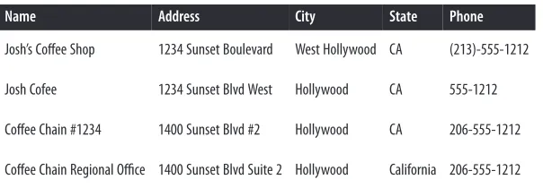
The general structure of the problem is something like this: we have a large collection of records from one or more source systems, and it is likely that some of the records refer to the same underlying entity, such as a customer, a patient, or the location of a business or an event. Each of the entities has a number of attributes, such as a name, an address, or a birthday, and we will need to use these attributes to find the records that refer to the same entity. Unfortunately, the values of these attributes aren’t per‐ fect: values might have different formatting, or typos, or missing information that means that a simple equality test on the values of the attributes will cause us to miss a significant number of duplicate records. For example, let’s compare the business list‐ ings shown in Table 2-1.
Table 2-1. The challenge of record linkage
Name Address City State Phone
Josh’s Coffee Shop 1234 Sunset Boulevard West Hollywood CA (213)-555-1212
Josh Cofee 1234 Sunset Blvd West Hollywood CA 555-1212
Coffee Chain #1234 1400 Sunset Blvd #2 Hollywood CA 206-555-1212
Coffee Chain Regional Office 1400 Sunset Blvd Suite 2 Hollywood California 206-555-1212
The first two entries in this table refer to the same small coffee shop, even though a data entry error makes it look as if they are in two different cities (West Hollywood versus Hollywood). The second two entries, on the other hand, are actually referring to different business locations of the same chain of coffee shops that happen to share a common address: one of the entries refers to an actual coffee shop, and the other one refers to a local corporate office location. Both of the entries give the official phone number of corporate headquarters in Seattle.
This example illustrates everything that makes record linkage so difficult: even though both pairs of entries look similar to each other, the criteria that we use to make the duplicate/not-duplicate decision is different for each pair. This is the kind of distinction that is easy for a human to understand and identify at a glance, but is difficult for a computer to learn.
Getting Started: The Spark Shell and SparkContext
We’re going to use a sample data set from the UC Irvine Machine Learning Reposi‐ tory, which is a fantastic source for a variety of interesting (and free) data sets for research and education. The data set we’ll be analyzing was curated from a record linkage study that was performed at a German hospital in 2010, and it contains sev‐ eral million pairs of patient records that were matched according to several different criteria, such as the patient’s name (first and last), address, and birthday. Each match‐ ing field was assigned a numerical score from 0.0 to 1.0 based on how similar the strings were, and the data was then hand-labeled to identify which pairs represented the same person and which did not. The underlying values of the fields themselves that were used to create the data set were removed to protect the privacy of the patients, and numerical identifiers, the match scores for the fields, and the label for each pair (match versus nonmatch) were published for use in record linkage research.
From the shell, let’s pull the data from the repository:
$ mkdir linkage $ cd linkage/
$ curl -o donation.zip http://bit.ly/1Aoywaq $ unzip donation.zip
$ unzip 'block_*.zip'
If you have a Hadoop cluster handy, you can create a directory for the block data in HDFS and copy the files from the data set there:
$ hadoop fs -mkdir linkage
$ hadoop fs -put block_*.csv linkage
The examples and code in this book assume you have Spark 1.2.1 available. Releases can be obtained from the Spark project site. Refer to the Spark documentation for instructions on setting up a Spark environment, whether on a cluster or simply on your local machine.
Now we’re ready to launch the spark-shell, which is a REPL (read-eval-print loop) for the Scala language that also has some Spark-specific extensions. If you’ve never seen the term REPL before, you can think of it as something similar to the R environ‐ ment: it’s a place where you can define functions and manipulate data in the Scala programming language.
If you have a Hadoop cluster that runs a version of Hadoop that supports YARN, you can launch the Spark jobs on the cluster by using the value of yarn-client for the Spark master:
$ spark-shell --master yarn-client
However, if you’re just running these examples on your personal computer, you can launch a local Spark cluster by specifying local[N], where N is the number of threads
to run, or * to match the number of cores available on your machine. For example, to launch a local cluster that uses eight threads on an eight-core machine:
$ spark-shell --master local[*]
The examples will work the same way locally. You will simply pass paths to local files, rather than paths on HDFS beginning with hdfs://. Note that you will still need to cp block_*.csv into your chosen local directory rather than use the directory con‐ taining files you unzipped earlier, because it contains a number of other files besides the .csv data files.
The rest of the examples in this book will not show a --master argument to spark-shell, but you will typically need to specify this argument as appropriate for your environment.
You may need to specify additional arguments to make the Spark shell fully utilize your resources. For example, when running Spark with a local master, you can use --driver-memory 2g to let the single local process use 2 gigabytes of memory. YARN memory configuration is more complex, and relevant options like --executor-memory are explained in the Spark on YARN documentation.
After running one of these commands, you will see a lot of log messages from Spark as it initializes itself, but you should also see a bit of ASCII art, followed by some additional log messages and a prompt:
Welcome to
____ __ / __/__ ___ _____/ /__ _\ \/ _ \/ _ `/ __/ '_/
/___/ .__/\_,_/_/ /_/\_\ version 1.2.1 /_/
Using Scala version 2.10.4
(Java HotSpot(TM) 64-Bit Server VM, Java 1.7.0_67) Type in expressions to have them evaluated.
Type :help for more information. Spark context available as sc. scala>
If this is your first time using the Spark shell (or any Scala REPL, for that matter), you should run the :help command to list available commands in the shell. :history and :h? can be helpful for finding the names that you gave to variables or functions that you wrote during a session but can’t seem to find at the moment. :paste can help you correctly insert code from the clipboard—something you may well want to do while following along with the book and its accompanying source code.
In addition to the note about :help, the Spark log messages indicated that “Spark context available as sc.” This is a reference to the SparkContext, which coordinates the execution of Spark jobs on the cluster. Go ahead and type sc at the command line:
sc
...
res0: org.apache.spark.SparkContext = org.apache.spark.SparkContext@DEADBEEF
The REPL will print the string form of the object, and for the SparkContext object, this is simply its name plus the hexadecimal address of the object in memory (DEAD BEEF is a placeholder; the exact value you see here will vary from run to run.)
It’s good that the sc variable exists, but what exactly do we do with it? SparkContext is an object, and as an object, it has methods associated with it. We can see what those methods are in the Scala REPL by typing the name of a variable, followed by a period, followed by tab: getExecutorStorageStatus getLocalProperty getPersistentRDDs getPoolForName
The SparkContext has a long list of methods, but the ones that we’re going to use most often allow us to create Resilient Distributed Datasets, or RDDs. An RDD is Spark’s fundamental abstraction for representing a collection of objects that can be
distributed across multiple machines in a cluster. There are two ways to create an RDD in Spark:
• Using the SparkContext to create an RDD from an external data source, like a file in HDFS, a database table via JDBC, or a local collection of objects that we create in the Spark shell.
• Performing a transformation on one or more existing RDDs, like filtering records, aggregating records by a common key, or joining multiple RDDs together.
RDDs are a convenient way to describe the computations that we want to perform on our data as a sequence of small, independent steps.
Resilient Distributed Datasets
An RDD is laid out across the cluster of machines as a collection of partitions, each including a subset of the data. Partitions define the unit of parallelism in Spark. The framework processes the objects within a partition in sequence, and processes multi‐ ple partitions in parallel. One of the simplest ways to create an RDD is to use the parallelize method on SparkContext with a local collection of objects:
val rdd = sc.parallelize(Array(1, 2, 2, 4), 4) ...
rdd: org.apache.spark.rdd.RDD[Int] = ...
The first argument is the collection of objects to parallelize. The second is the number of partitions. When the time comes to compute the objects within a partition, Spark fetches a subset of the collection from the driver process.
To create an RDD from a text file or directory of text files residing in a distributed filesystem like HDFS, we can pass the name of the file or directory to the textFile method:
val rdd2 = sc.textFile("hdfs:///some/path.txt") ...
rdd2: org.apache.spark.rdd.RDD[String] = ...
When you’re running Spark in local mode, the textFile method can access paths that reside on the local filesystem. If Spark is given a directory instead of an individ‐ ual file, it will consider all of the files in that directory as part of the given RDD. Finally, note that no actual data has been read by Spark or loaded into memory yet, either on our client machine or the cluster. When the time comes to compute the objects within a partition, Spark reads a section (also known as a split) of the input file, and then applies any subsequent transformations (filtering, aggregation, etc.) that we defined via other RDDs.
Our record linkage data is stored in a text file, with one observation on each line. We will use the textFile method on SparkContext to get a reference to this data as an RDD:
val rawblocks = sc.textFile("linkage") ...
rawblocks: org.apache.spark.rdd.RDD[String] = ...
There are a few things happening on this line that are worth going over. First, we’re declaring a new variable called rawblocks. As we can see from the shell, the raw blocks variable has a type of RDD[String], even though we never specified that type information in our variable declaration. This is a feature of the Scala programming language called type inference, and it saves us a lot of typing when we’re working with the language. Whenever possible, Scala figures out what type a variable has based on its context. In this case, Scala looks up the return type from the textFile function on the SparkContext object, sees that it returns an RDD[String], and assigns that type to the rawblocks variable.
Whenever we create a new variable in Scala, we must preface the name of the variable with either val or var. Variables that are prefaced with val are immutable, and can‐ not be changed to refer to another value once they are assigned, whereas variables that are prefaced with var can be changed to refer to different objects of the same type. Watch what happens when we execute the following code:
rawblocks = sc.textFile("linkage") ...
<console>: error: reassignment to val
var varblocks = sc.textFile("linkage")
varblocks = sc.textFile("linkage")
Attempting to reassign the linkage data to the rawblocks val threw an error, but reassigning the varblocks var is fine. Within the Scala REPL, there is an exception to the reassignment of vals, because we are allowed to redeclare the same immutable variable, like the following:
val rawblocks = sc.textFile("linakge")
val rawblocks = sc.textFile("linkage")
In this case, no error is thrown on the second declaration of rawblocks. This isn’t typ‐ ically allowed in normal Scala code, but it’s fine to do in the shell, and we will make extensive use of this feature throughout the examples in the book.
The REPL and Compilation
In addition to its interactive shell, Spark also supports compiled applications. We typ‐ ically recommend using Maven for compiling and managing dependencies. The Git‐ Hub repository included with this book holds a self-contained Maven project setup under the simplesparkproject/ directory to help you with getting started.
With both the shell and compilation as options, which should you use when testing out and building a data pipeline? It is often useful to start working entirely in the REPL. This enables quick prototyping, faster iteration, and less lag time between ideas and results. However, as the program builds in size, maintaining a monolithic file of code become more onerous, and Scala interpretation eats up more time. This can be exacerbated by the fact that, when you’re dealing with massive data, it is not uncom‐ mon for an attempted operation to cause a Spark application to crash or otherwise render a SparkContext unusable. This means that any work and code typed in so far becomes lost. At this point, it is often useful to take a hybrid approach. Keep the fron‐ tier of development in the REPL, and, as pieces of code harden, move them over into a compiled library. You can make the compiled JAR available to spark-shell by pass‐ ing it to the --jars property. When done right, the compiled JAR only needs to be rebuilt infrequently, and the REPL allows for fast iteration on code and approaches that still need ironing out.
What about referencing external Java and Scala libraries? To compile code that refer‐ ences external libraries, you need to specify the libraries inside the project’s Maven configuration (pom.xml). To run code that accesses external libraries, you need to include the JARs for these libraries on the classpath of Spark’s processes. A good way to make this happen is to use Maven to package a JAR that includes all of your appli‐ cation’s dependencies. You can then reference this JAR when starting the shell by using the --jars property. The advantage of this approach is the dependencies only need to be specified once: in the Maven pom.xml. Again, the simplesparkproject/
directory in the GitHub repository shows you how to accomplish this.
SPARK-5341 also tracks development on the capability to specify Maven repositories directly when invoking spark-shell and have the JARs from these repositories auto‐ matically show up on Spark’s classpath.
Bringing Data from the Cluster to the Client
RDDs have a number of methods that allow us to read data from the cluster into the Scala REPL on our client machine. Perhaps the simplest of these is first, which returns the first element of the RDD into the client:
rawblocks.first
...
res: String = "id_1","id_2","cmp_fname_c1","cmp_fname_c2",...
The first method can be useful for sanity checking a data set, but we’re generally interested in bringing back larger samples of an RDD into the client for analysis. When we know that an RDD only contains a small number of records, we can use the collect method to return all of the contents of an RDD to the client as an array. Because we don’t know how big the linkage data set is just yet, we’ll hold off on doing this right now.
We can strike a balance between first and collect with the take method, which allows us to read a given number of records into an array on the client. Let’s use take to get the first 10 lines from the linkage data set:
val head = rawblocks.take(10) ...
head: Array[String] = Array("id_1","id_2","cmp_fname_c1",...
head.length
...
res: Int = 10
Actions
The act of creating an RDD does not cause any distributed computation to take place on the cluster. Rather, RDDs define logical data sets that are intermediate steps in a computation. Distributed computation occurs upon invoking an action on an RDD. For example, the count action returns the number of objects in an RDD:
rdd.count()
14/09/10 17:36:09 INFO SparkContext: Starting job: count ...
14/09/10 17:36:09 INFO SparkContext: Job finished: count ... res0: Long = 4
The collect action returns an Array with all the objects from the RDD. This Array resides in local memory, not on the cluster:
rdd.collect()
14/09/29 00:58:09 INFO SparkContext: Starting job: collect ...
14/09/29 00:58:09 INFO SparkContext: Job finished: collect ... res2: Array[(Int, Int)] = Array((4,1), (1,1), (2,2))
Actions need not only return results to the local process. The saveAsTextFile action saves the contents of an RDD to persistent storage, such as HDFS:
rdd.saveAsTextFile("hdfs:///user/ds/mynumbers")
14/09/29 00:38:47 INFO SparkContext: Starting job:
saveAsTextFile ...
14/09/29 00:38:49 INFO SparkContext: Job finished:
saveAsTextFile ...
The action creates a directory and writes out each partition as a file within it. From the command line outside of the Spark shell:
hadoop fs -ls /user/ds/mynumbers
-rw-r--r-- 3 ds supergroup 0 2014-09-29 00:38 myfile.txt/_SUCCESS -rw-r--r-- 3 ds supergroup 4 2014-09-29 00:38 myfile.txt/part-00000 -rw-r--r-- 3 ds supergroup 4 2014-09-29 00:38 myfile.txt/part-00001
Remember that textFile can accept a directory of text files as input, meaning that a future Spark job could refer to mynumbers as an input directory.
The raw form of data that is returned by the Scala REPL can be somewhat hard to read, especially for arrays that contain more than a handful of elements. To make it easier to read the contents of an array, we can use the foreach method in conjunction with println to print out each value in the array on its own line:
head.foreach(println) ...
"id_1","id_2","cmp_fname_c1","cmp_fname_c2","cmp_lname_c1","cmp_lname_c2", "cmp_sex","cmp_bd","cmp_bm","cmp_by","cmp_plz","is_match"
37291,53113,0.833333333333333,?,1,?,1,1,1,1,0,TRUE
39086,47614,1,?,1,?,1,1,1,1,1,TRUE
70031,70237,1,?,1,?,1,1,1,1,1,TRUE
84795,97439,1,?,1,?,1,1,1,1,1,TRUE
36950,42116,1,?,1,1,1,1,1,1,1,TRUE
42413,48491,1,?,1,?,1,1,1,1,1,TRUE
25965,64753,1,?,1,?,1,1,1,1,1,TRUE
49451,90407,1,?,1,?,1,1,1,1,0,TRUE
39932,40902,1,?,1,?,1,1,1,1,1,TRUE
The foreach(println) pattern is one that we will frequently use in this book. It’s an example of a common functional programming pattern, where we pass one function (println) as an argument to another function (foreach) in order to perform some action. This kind of programming style will be familiar to data scientists who have worked with R and are used to processing vectors and lists by avoiding for loops and instead using higher-order functions like apply and lapply. Collections in Scala are similar to lists and vectors in R in that we generally want to avoid for loops and instead process the elements of the collection using higher-order functions.
Immediately, we see a couple of issues with the data that we need to address before we begin our analysis. First, the CSV files contain a header row that we’ll want to filter out from our subsequent analysis. We can use the presence of the "id_1" string in the row as our filter condition, and write a small Scala function that tests for the presence of that string inside of the line:
def isHeader(line: String) = line.contains("id_1")
isHeader: (line: String)Boolean
Like Python, we declare functions in Scala using the keyword def. Unlike Python, we have to specify the types of the arguments to our function; in this case, we have to indicate that the line argument is a String. The body of the function, which uses the contains method for the String class to test whether or not the characters "id_1" appear anywhere in the string, comes after the equals sign. Even though we had to specify a type for the line argument, note that we did not have to specify a return type for the function, because the Scala compiler was able to infer the type based on its knowledge of the String class and the fact that the contains method returns true or false.
Sometimes, we will want to specify the return type of a function ourselves, especially for long, complex functions with multiple return statements, where the Scala com‐ piler can’t necessarily infer the return type itself. We might also want to specify a return type for our function in order to make it easier for someone else reading our code later to be able to understand what the function does without having to reread the entire method. We can declare the return type for the function right after the argument list, like this:
def isHeader(line: String): Boolean = { line.contains("id_1")
}
isHeader: (line: String)Boolean
We can test our new Scala function against the data in the head array by using the filter method on Scala’s Array class and then printing the results:
head.filter(isHeader).foreach(println) ...
"id_1","id_2","cmp_fname_c1","cmp_fname_c2","cmp_lname_c1",...
It looks like our isHeader method works correctly; the only result that was returned from applying it to the head array via the filter method was the header line itself. But of course, what we really want to do is get all of the rows in the data except the header rows. There are a few ways that we can do this in Scala. Our first option is to take advantage of the filterNot method on the Array class:
head.filterNot(isHeader).length
...
res: Int = 9
We could also use Scala’s support for anonymous functions to negate the isHeader function from inside filter:
head.filter(x => !isHeader(x)).length
...
res: Int = 9
Anonymous functions in Scala are somewhat like Python’s lambda functions. In this case, we defined an anonymous function that takes a single argument called x and
passes x to the isHeader function and returns the negation of the result. Note that we did not have to specify any type information for the x variable in this instance; the Scala compiler was able to infer that x is a String from the fact that head is an Array[String].
There is nothing that Scala programmers hate more than typing, so Scala has lots of little features that are designed to reduce the amount of typing they have to do. For example, in our anonymous function definition, we had to type the characters x => in order to declare our anonymous function and give its argument a name. For simple anonymous functions like this one, we don’t even have to do that; Scala will allow us to use an underscore (_) to represent the argument to the anonymous function, so that we can save four characters:
head.filter(!isHeader(_)).length
...
res: Int = 9
Sometimes, this abbreviated syntax makes the code easier to read because it avoids duplicating obvious identifiers. Sometimes, this shortcut just makes the code cryptic. The code listings use one or the other according to our best judgment.
Shipping Code from the Client to the Cluster
We just saw a wide variety of ways to write and apply functions to data in Scala. All of the code that we executed was done against the data inside the head array, which was contained on our client machine. Now we’re going to take the code that we just wrote and apply it to the millions of linkage records contained in our cluster and repre‐ sented by the rawblocks RDD in Spark.
Here’s what the code looks like to do this; it should feel eerily familiar to you:
val noheader = rawblocks.filter(x => !isHeader(x))
The syntax that we used to express the filtering computation against the entire data set on the cluster is exactly the same as the syntax we used to express the filtering computation against the array of data in head on our local machine. We can use the first method on the noheader RDD to verify that the filtering rule worked correctly:
noheader.first
...
res: String = 37291,53113,0.833333333333333,?,1,?,1,1,1,1,0,TRUE
This is incredibly powerful. It means that we can interactively develop and debug our data-munging code against a small amount of data that we sample from the cluster, and then ship that code to the cluster to apply it to the entire data set when we’re ready to transform the entire data set. Best of all, we never have to leave the shell. There really isn’t another tool that gives you this kind of experience.
In the next several sections, we’ll use this mix of local development and testing and cluster computation to perform more munging and analysis of the record linkage data, but if you need to take a moment to drink in the new world of awesome that you have just entered, we certainly understand.
Structuring Data with Tuples and Case Classes
Right now, the records in the head array and the noheader RDD are all strings of comma-separated fields. To make it a bit easier to analyze this data, we’ll need to parse these strings into a structured format that converts the different fields into the correct data type, like an integer or double.
If we look at the contents of the head array (both the header line and the records themselves), we can see the following structure in the data:
• The first two fields are integer IDs that represent the patients that were matched in the record.
• The next nine values are (possibly missing) double values that represent match scores on different fields of the patient records, such as their names, birthdays, and location.
• The last field is a boolean value (TRUE or FALSE) indicating whether or not the pair of patient records represented by the line was a match.
Like Python, Scala has a built-in tuple type that we can use to quickly create pairs, triples, and larger collections of values of different types as a simple way to represent records. For the time being, let’s parse the contents of each line into a tuple with four values: the integer ID of the first patient, the integer ID of the second patient, an array of nine doubles representing the match scores (with NaN values for any missing fields), and a boolean field that indicates whether or not the fields matched.
Unlike Python, Scala does not have a built-in method for parsing comma-separated strings, so we’ll need to do a bit of the legwork ourselves. We can experiment with our parsing code in the Scala REPL. First, let’s grab one of the records from the head array:
val line = head(5)
val pieces = line.split(',') ...
pieces: Array[String] = Array(36950, 42116, 1, ?,...
Note that we accessed the elements of the head array using parentheses instead of brackets; in Scala, accessing array elements is a function call, not a special operator. Scala allows classes to define a special function named apply that is called when we treat an object as if it were a function, so head(5) is the same thing as head.apply(5).