Presentation Iso31010 v02 Quantitative

(1)

(2)

Daftar Isi

• Asesmen risiko dalam kerangka kerja dan

proses manajemen risiko ISO31000

• Seleksi teknik-teknik asesmen risiko:

– Identifikasi risiko – Analisis risiko

– Evaluasi risiko

• Teknik asesmen risiko berbasis non-statistik

(3)

Modul 4-1

• STATISTICAL METHODS FOR RISK ASSESSMENT

THE SCIENCE OF DATA

RISK ASSESSMENT TECHNIQUES

IEC / ISO 31010

(4)

• Statistika adalah ilmu tentang data.

• Statistika deskriptif: menggunakan metode

numerik dan grafik untuk mencari pola dari sekumpulan data, dan menyajikan informasi tentang pola tersebut dengan cara tertentu.

• Statistika inferensial: membuat estimasi tentang

nilai yang akan terjadi atau generalisasi bagi

populasi berdasarkan informasi yang diperoleh dari sejumlah data yang tersedia (sampel).

(5)

Sejumlah metode statistika dapat dipakai untuk:

• mengestimasi besarnya probabilitas dan/atau

dampak dari suatu risiko (analisa risiko).

• menguji keandalan hasil estimasi (identifikasi

risiko)

• merevisi hasil estimasi dengan diperolehnya

informasi baru (informasi untuk evaluasi risiko)

(6)

• Data diperoleh dari mengukur variabel.

• Data berupa angka dapat bersifat kuantitatif atau kualitatif.

• Angka yang kualitatif adalah hasil dari pengukuran dengan skala nominal dan ordinal, angka yang

benar-benar kuantitatif dihasilkan dari pengukuran dengan skala interval dan rasio.

• Perlakuan matematis yang dapat diterapkan atas kedua jenis angka tersebut berbeda.

(7)

(8)

Data dapat disajikan

• sebagai deretan angka,

• dalam tabel (tabel distribusi frekuensi), atau

• dengan gambar (histogram, diagram batang,

pie chart, distribusi probabilitas)

(9)

Mendeskripsikan data adalah menguraikan pola data menurut tiga ukuran: kecenderungan

memusat, dispersi, dan posisi relatif.

• Measures of central tendency: mean, median, mode

• Measures of dispersion: range, variance, standard deviation

• Measures of relative standing: skewness, curtosis

(10)

QUANTITATIVE DATA

Hasil pengukuran atas usia (tahun) dari 7 pegawai di

sebuah perusahaan jasa komputer adalah: 20, 25, 34, 35, 35, 36, 40 Mean = Median = 35 Mode = 35 Range = (max-min) = 40-20 = 20 Varians = Standar deviasi = Skewness =

(11)

QUALITATIVE DATA

Sebanyak 20 nasabah menyampaikan kepuasan mereka atas

layanan petugas bank. Ada 1 nasabah menyatakan tidak puas, 10 nasabah menyatakan cukup puas, dan sisanya menyatakan puas.

Kecenderungan memusat: Sebaran:

Kepuasan Frekuensi mutlak Frekuensi relatif

Tidak puas 1 5 %

Cukup puas 10 50 %

(12)

Modul 4-2

PROBABILITY

RISK ASSESSMENT TECHNIQUES

IEC / ISO 31010

(13)

PROBABILITY THEORY

 0 ≤ P(A_i) ≤ 1 untuk tiap peristiwa A_i dalam sampel S  P(A_i) = 1 – P(A_ic)

 P(A₁∩A₂) = 0 if A₁ dan A₂mutually exclusive

 P(A₁∩A₂) = P(A₁) x P(A₂) if A₁ dan A₂independent  P(A₁∪A₂) = P(A₁) + P(A₂) - P(A₁∩A₂)

Dari pelemparan dadu sebayak satu kali: P (1) = P (mendapat mata 1) =

P (1c_{) = (mendapat mata bukan 1) =}

P (1 ∩ 2) = P (1 ∪ 2) =

(14)

CONDITIONAL, UNCONDITIONAL, AND JOINT PROBABILITIES

• Unconditional probability P(A) = Probability of event A to occur

• Conditional probability P(A|B) = Probability of A given B has occurred

• Joint probability P (A ∩ B) = P(A) x P(B|A) = P(A|B) x P(B)

(15)

EXERCISE OF CONDITIONAL, UNCONDITIONAL, AND JOINT PROBABILITIES

• Suppose that the eye color of students in a class of 40 people as follows;

• Events:

A: Selecting a Male student.

B: Selecting a student with Black Eyes. C: Selecting a Female student.

(16)

• Q1. If the selected student is a Male student, what is the probability that he has got Green Eyes?

• Q2. If the selected student is a Female student, what is the probability that she has got Green Eyes?

(17)

• Q1

P(D|A) = P(DA) / P(A) = (8/40) / (28/40) = 0.074

• Q2

(18)

BAYES’ INFERENTIAL METHOD

• Informasi tentang probabilitas perlu dan dapat

diperbaiki bila probabilitas bersifat subyektif.

• Bayes’ rule menunjukkan bagaimana

probabilitas terjadinya suatu peristiwa berubah bila ada informasi baru yang terkait dengan

peristiwa yang sedang menjadi perhatian.

• Bayes’ rule: menggunakan prior probabilities of

event A, B, dan BA untuk mendapatkan probabilitas AB

(19)

EXERCISE 1

• Economists believe that the annual inflation rate in Turkey is affected by the changes in the petroleum prices. The probability of inflation rate increasing in 2001 is estimated to be 0.60. The probability of

petroleum prices rising is 0.40. The probability of

both inflation rate and the petroleum prices rising is 0.35. On the other hand, the probability of inflation rate rising and at the same time, the petroleum

prices not rising is estimated to be 0.20. If

petroleum prices do not rise in 2001, what is the probability of inflation rate rising?

(20)

SOLUTION: EXERCISE 1

Events: I: Inflation rate increasing. P: Petroleum prices rising. N: Petroleum prices not rising

Given: P(I) = 0.6 P(P) = 0.4 P(IP) = 0.35 P(IN) = 0.2 Solution: P(N) = 1 – P(P) = 1- 0.4 = 0.6 P(I | N) = P(IN) / P(N) = 0.2 / 0.6 = 0.333 ≈ 0.3

(21)

EXERCISE 2

• Annual profits of construction sector depend on wage rate paid to labor employed by the sector. The past data about the behavior of annual profits suggested that the probability of profits rising in a given year is 0.80 and the probability of

profits falling is 0.20. The past data also suggest that in 60% of all the years during which the profits have increased, wage

rate has declined, and it has increased in the remaining 40%. However, in 80% of all years during which profits have fallen, wage rate has increased, and the only remaining 20% wage rate has decreased. Due to the economic crisis in Turkey, wage rate has been declining since the beginning of 2005. Given this downward trend in wages, what is our revised estimate for the probability of annual profits of construction sector to rise in the year?

(22)

Events: A: Profits rising

B: Profits falling

C: Wage rate declining D: Wage rate increasing Given: P(A) = 0.80 P(B) = 0.20 P(C|A) = 0.60 P(D|A) = 0.40 P(D|B) = 0.80 P(C|B) = 0.20

(23)

Solution: Without using the table

P(A|C) = P(AC) / P(C) or P(CA) / P(A) 0.60 = P(CA) / 0.80 P(CA) or P(AC) = 0.60 * 0.80 = 0.48 P(C) = P(CA) + P(CB) = [P(C|A) * P(A)] + [P(C/B) * P(B)] = (0.60 * 0.80) + (0.20 * 0.20) = 0.48 + 0.04 = 0.52 P(A|C) = 0.48 / 0.52 = 0.92

(24)

Modul 4-3

MARKOV ANALYSIS

RISK ASSESSMENT TECHNIQUES

IEC / ISO 31010

(25)

MARKOV INFERENTIAL METHOD

• Situasi: sederetan peristiwa, satu setelah yang lain. Cuaca hari ini dipengaruhi cuaca kemarin, ketrampilan seseorang pada minggu ini ditentukan oleh tingkat ketrampilan yang dimilikinya minggu lalu.

• Markov model mengasumsikan bahwa masa yang akan datang tidak lagi ditentukan oleh masa lalu ketika masa sekarang telah diperhitungkan.

• Markov method adalah suatu teknik yang menggunakan

informasi yang ada sampai pada saat estimasi, mengestimasi berbagai kemungkinan yang dapat terjadi pada masa yang akan datang dengan probabilitas dari setiap peristiwa yang mungkin terjadi.

(26)

Example of Markov’ Managerial Problem

• Dalam sebuah industri terdapat sejumlah perusahaan yang bersaing satu dengan yang lain. Pangsa pasar dari semua perusahaan yang ada di industri tersebut pada setiap waktu tertentu, misalnya awal bulan, merupakan informasi publik. Berdasarkan informasi dari waktu ke waktu, bagi setiap

perusahaan dapat dihitung probabilitas perusahaan tersebut berubah pangsa pasarnya. Untuk kepentingan menentukan target atau bahkan tujuan perusahaan, dapat disediakan perkiraan tentang pangsa pasar yang dapat dicapai

perusahaan dan probabilitas untuk mencapai target tersebut. • Berdasarkan informasi tentang pangsa pasar sekarang,

estimasikan berapa pangsa pasar yang akan terjadi pada waktu yang akan datang dan berapa probabilitas itu untuk tercapai.

(27)

States and State Probabilities

• States: all possible conditions of a process or system • In Markov analysis it is assumed that the states are

both collectively exhaustive and mutually exclusive

• Pada setiap waktu i, ada n states, dengan probabilitas

P(i) = (P_i1, P_i2, P_i3, … , P_in)

Untuk periode waktu sepanjang m, matriks transisi Markov adalah

(28)

Matrix of Transition Probabilities P = P₁₁ P₁₂ P₁₃ … P_1n P₂₁ P₂₂ P₂₃ … P_2n Pm1 Pmn … … …

 P_ij = conditional probability of being in state j in the future given i as the

current state

 Individual P_ij values are determined empirically  The probabilities in each row will sum to 1

(29)

Example of Markov’s estimation on market share

Tiga perusahaan, C₁, C₂, dan C₃ mempunyai pangsa pasar masing-masing 0,4, 0,3, dan 0,3. Dengan mengandaikan bahwa ada tiga states (situasi pangsa pasar yang mungkin), matriks transisi untuk pindah dari pangsa pasar sekarang ke pangsa pasar yang akan datang adalah

P =

0.8 0.1 0.1

0.1 0.7 0.2

0.2 0.2 0.6

Baris 1

0.8 = P₁₁ = probabilitas pindah dari state 1 ke state 1

0.1 = P₁₂ = probabilitas untuk pindah dari state 1 ke state 2 0.1 = P₁₃ = probabilitas untuk pindah dari state 1 ke state 3

(30)

Predicting Future Market Shares

• When the current period is 0, the state probabilities for the period 1 are determined as

π (1) = π (0) x P

 For any period n we can compute the state probabilities for period n + 1

(31)

 When the current period is 0, and 1 is the next period, the

state probabilities for the period 1

π (1) = π (0) x P = (0.4, 0.3, 0.3) 0.8 0.1 0.1 0.1 0.7 0.2 0.2 0.2 0.6 = [(0.4)(0.8) + (0.3)(0.1) + (0.3)(0.2), (0.4)(0.1) + (0.3)(0.7) + (0.3)(0.2), (0.4)(0.1) + (0.3)(0.2) + (0.3)(0.6)] = (0.41, 0.31, 0.28)

(32)

 Masuk ke priode 1, diperkirakan pangsa pasar C₁

dan C₂ meningkat, sedangkan pangsa pasar C₃ turun.

 Estimasi dapat dilakukan untuk periode 2 dst.  Setiap akhir periode akan ada data baru tentang

pangsa pasar yang nyata terjadi (state yang

sesungguhnya dari setiap perusahaan). Matriks transisi P biasanya diasumsikan konstan (tidak berubah dengan berubahnya waktu)

(33)

Modul 4-4

DISTRIBUTION

RISK ASSESSMENT TECHNIQUES

IEC / ISO 31010

(34)

Discrete and Continuous Distribution

Discrete:

•The data is commonly divided into intervals or groups

•The number of members for every group can counted

Continuous:

•Commonly divided into ranges •The number of members for a range cannot be counted

•Types: uniform, normal, t-distribution, log normal, Chi

(35)

Discrete Distribution: The Binomial Distribution

• Binomial defined as the number of “successes” in a given number of trials, whereby the outcome can be either success or failure

• Probability of success, p, is constant for each trial.

• The final outcome is the number of successes in a series of n trials.

• Binomial probability function is the probability of x successes in n trials.

x n x x n C p p x P( )= (1 − ) − P X n x n x p p x n x ( ) ! !( )! ( ) = − − − 1 OR Combination: The number of ways x can

happen . px_{: the probability of} success compounded by x times of success (1 –p)n-x : the probability of failure compounded by n-x times of failure

(36)

36

Example Binomial Distribution

• Football Team is competing for league

championship. Probability of winning in any match is 0.6. What is the probability of

winning 3 times during the next 5 matches?

• Answer : ) 6 . 0 1 ( 6 . 0 )! 3 5 ( ! 3 ! 5 ) 3 ( ) 1 ( )! ( ! ! ) ( 3 5 3 = − − = = − − = − − X P p p x n x n X P x n x

(37)

P X x x ( ) ! = e-λ λ P(X) = Probability of X ‘successes’

λ ₌ _{Expected (mean) number of ‘successes’}

e = 2.71828 (base of natural logs)

x = Number of ‘successes’ per unit

.4 .6 P(X) λ = 0.5 λ = 6 µ λ σ λ = = = = = ∑ E X X P X_i i N i ( ) ( ) 1 Mean Standard Deviation

(38)

• Poisson Distribution is calculating the probability of getting a result which is usually different from the standard result.

• Usually used in quality control and risk management for calculating the probability of getting a result which is different from the

predefined standard

• Number of events that occur in an area of opportunity – Events per unit

• Example: Time, length, area, space • Examples

– # customers arriving in 20 minutes – # strikes per year in the U.S.

– # defects per lot (group) of VCR's

(39)

• X is uniformly distributed between 2 and 12. Calculate the probability that X will be between 4 and 8

Example Continuous Uniform Distribution

Probability

x

2 4 ₈ 12

(40)

• Continuous uniform distribution is defined over a range that spans between some lower limit, a, and some upper limit, b, which serve as the parameters of the distribution.

• Outcomes can only occur between a and b

• A random variable is uniformly distributed whenever the probability is proportional to the interval’s length.

• Uniform Probability Density Function

f(x) = 1/(b - a) for a < x < b = 0 elsewhere

where: a = smallest value the variable can assume b = largest value the variable can assume

(41)

Characteristics of the Normal Probability Distribution

• Two parameters, µ (mean) and σ (standard deviation), completely describe the location and shape of the distribution.

• Skewness = 0, normal distribution is symmetric about its mean about its mean, so probability above and below the mean is 50%

• Kurtosis = 3

• The shape of the normal curve is often illustrated as a bell-shaped curve.

• The highest point on the normal curve is at the mean, which is also the median and mode. • The mean can be any numerical value: negative, zero, or positive.

• Probabilities for the normal random variable are given by areas under the curve.

The probabilities of outcomes further above and below the mean get smaller but do not go to

NORMAL PROBABILITY DISTRIBUTION

Theoretically, the curve extends to -∞

Theoretically, the curve extends to ∞ The normal curve is symmetrical, the two halves are identical

(42)

(43)

Lognormal Distribution

• Generated by the function of ex, where x is normally distributed.

Since the natural logarithm, ln, of ex_{is x, logarithm of lognormally}

distributed variables are normally distributed • Skewed to the right

• Bounded from below by zero so useful for modelling asset price with no negative values.

(44)

(45)

Exponential Distribution

• Exponential Distribution is widely used to model waiting times.

• In risk management it is used as model to provide a time weight

of a series of data to capture the level of obsolescence of older data entry by giving it lower weight than the newer ones.

• F(x) = 1 / β X e-x/β, x ≥ 0

• β is the scale parameter which is greater than 0 and reciprocal of

rate parameter l (i.e. l = 1 / β).

• In context of waiting for company to default, the rate parameter

is the hazard rate, and indicates the rate at which default will arrive

(46)

(47)

Chi Square Distribution

• Used to evaluate the variance of a normally

distributed random variable

• It is bounded by zero.

• Chi Square is asymmetrical and approaches

normal distribution shape as degrees of freedom increase

(48)

(49)

T Distribution

• Symmetrical distribution which is centered

about zero

• The shape depends on the number of degrees

of freedom which is based on the number of observations

• Flatter and thicker than normal distribution

• When number of observations increases, the

(50)

(51)

Triangle Distribution

• The Triangle distribution is used as a rough modeling tool where the range (a to c) and the most likely value within the range (b) can be estimated. Its statistical properties are derived from from its geometry.

• This distribution offers considerable flexibility in its shape,

coupled with the intuitive nature of its defining parameters and speed of use. However, a and c are the absolute minimum and maximum estimated values for the variable and it is difficult to estimates these values.

• Triangle shape overemphasize the tails of the distribution and under emphasize the shoulders in comparison with other, more natural, distributions.

(52)

Logistic Distribution

• The Logistic distribution looks similar to the Normal distribution but has a kurtosis of 4.2 compared to the Normal kurtosis of 3.

• The Logistic distribution is popular in demographic and economic modeling because it is similar to the Normal distribution but somewhat more peaked. It

(53)

(54)

Modul 5

Monte Carlo Simulation

RISK ASSESSMENT TECHNIQUES

IEC / ISO 31010

(55)

AGENDA

SIMULASI MONTE CARLO

CASE 1 SOFTWARE @RISK CASE 2 1 2 3 4 

(56)

SIMULASI MONTE CARLO

• Simulasi Monte Carlo adalah teknik komputerisasi matematis yang dilakukan untuk menghitung secara kuantitatif faktor risiko dan pengambilan keputusan.

• Simulasi Monte Carlo menghasilkan analisa risiko dari sebuah model yang dibangun dengan mengganti sebuah parameter dengan suatu rentang nilai – distribusi probabilitas – yang memiliki faktor

ketidakpastian. Kemudian dilakukan perhitungan berulang, masing-masing parameter dengan menggunakan suatu nilai acak (fungsi random) yang muncul dari sebuah fungsi distribusi

• Simulasi Monte Carlo bisa menghasilkan ribuan bahkan ratusan ribu perhitungan ulang, sampai

didapatkan hasil akhirnya. Semua bergantung pada tingkat ketidakpatian dan range data yang digunakan. • Simulasi Monte Carlo pertama kali ditemukan oleh John Von Nuemann, Stanislaw Ulam & Nicholas Metropolis pada tahun 1940 ketika mereka bekerja di Los Alamos National

(57)

DIBALIK NAMA MONTE CARLO

Monte Carlo adalah sebuah Casino di daerah Monte Carlo, Monaco yang terkenal dengan kompleks perjudian dan hiburan.

Simulasi Monte Carlo merupakan nama yang diberikan oleh Stanislaw Ulam untuk mengingat pamannya yang sering bermain kasino disana.

(58)

IEC/ISO 31010 RISK MANAGEMENT RISK ASSESSMENT TECHNIQUE

Simulasi MC

merupakan salah satu teknik assessment

risiko ISO 31000 yang dapat dipergunakan pada Risk Evaluation Terkait erat dengan prinsip no 3

(59)

IEC/ISO 31010 RISK MANAGEMENT

RISK ASSESSMENT TECHNIQUE

(60)

(61)

(62)

SIMULASI MONTE CARLO CASE 1 SOFTWARE @RISK CASE 2 1 2 3 4

(63)

INSTALASI SOFTWARE

• Software yang akan digunakan adalah

Palisade @RISK, sebuah program excel add-in

yang memungkinkan excel untuk melakukan simulasi monte carlo yang lebih advance

• Persyaratan minimum untuk instalasi

– PC setara Pentium

– Microsoft Windows 2000 SP4, Windows XP – Microsoft Excel 2000

(64)

INSTALASI SOFTWARE

• Microsoft Office memiliki pengaturan keamanan

terhadap Macro (Tools>Macro>Security) untuk menjaga agar Macro yang berbahaya tidak berfungsi di aplikasi Microsoft Office

• Versi percobaan @RISK adalah 15 hari jika software tidak diaktivasi

(65)

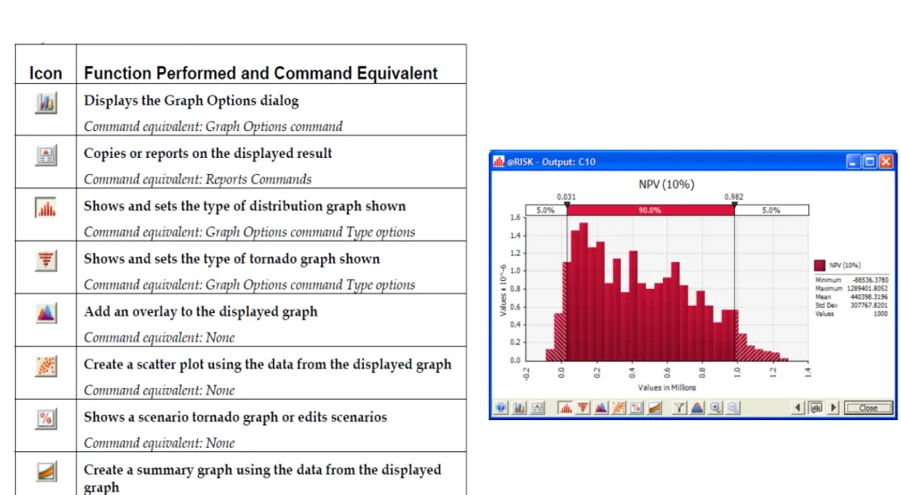
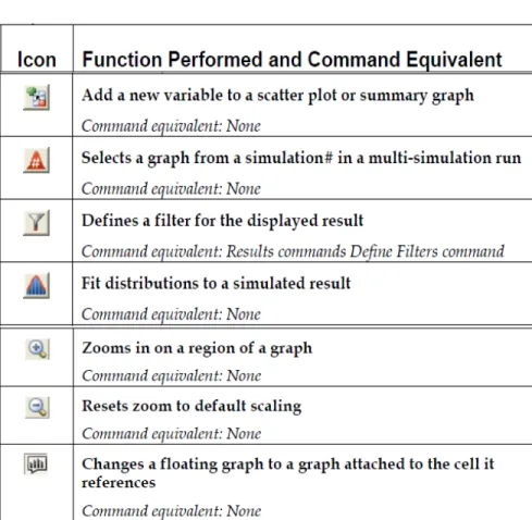
@RISK TOOLBAR

• Toolbar model: terdiri dari ikon-ikon untuk

membuat model dengan @RISK

• Toolbar simulasi: terdiri dari ikon-ikon untuk

(66)

@RISK TOOLBAR

• Toolbar hasil: terdiri dari ikon-ikon untuk melihat tampilan output dari model

• Toolbar alat bantu: terdiri dari ikon-ikon untuk

(67)

LANGKAH PENGGUNAAN SOFTWARE

Input (random variable)

Simulasi

(68)

LANGKAH CEPAT

• Buka Program Palisade @RISK

• Buka lembar kerja yang ingin disimulasikan

• Ganti cell excel yang berisi asumsi

deterministik menjadi asumsi stokastik dengan menambahkan distribusi @RISK

• Pilih cell yang akan dijadikan target dan klik

ikon “Add Output” pada toolbar @RISK

(69)

MEMASUKKAN UNSUR

KETIDAKPASTIAN

(70)

HASIL SIMULASI

• Menampilkan detail statistik

• List random data yang dipergunakan setiap

kali iterasi

• Analisa Sensitivitas simulasi dengan melihat

hubungan antara Y dengan X

• Berbagai skenario dari hasil simulasi

(71)

(72)

(73)

SIMULASI MONTE CARLO CASE 1 SOFTWARE @RISK CASE 2 1 2 3 4 

(74)

(75)

(76)

(77)

(78)

CASE #1 - SOLUTION

Lakukan langkah

Seperti gambar di samping

(79)

CASE #1 - SOLUTION

Lakukan langkah

Seperti gambar di samping

2

3

• Lakukan langkah seperti gambar di samping • Letakkan kursor pada cell A25

(80)

CASE #1 - SOLUTION

4

• Muncul box seperti gambar disamping • Pilih Columns

• Pada kotak Stop value isi 500 • Klik ok

(81)

CASE #1 - SOLUTION

5

• Letakkan kursor pada cell B25 • Ketik formula:

=B16+RAND()*(B17-B16)

• Letakkan kursor disebelah kiri B16, lalu tekan F4

• Lakukan langkah sebelumnya pada B17 dan B16

• Tekan Enter

• Isi cell B26:B524 dengan copy formula B25

(82)

CASE #1 - SOLUTION

6

• Letakkan kursor pada cell C25 • Ketik formula:

=BINOMDIST(B18,B19,B25,FALSE) • Tekan enter

(83)

CASE #1 - SOLUTION

• Data driven diagram – Line

diagram 7

• Letakkan kursor pada cell D25 • Ketik formula:

=BINOMDIST(C18,C19,B25,FALSE) • Tekan enter

• Letakkan kursor disebelah kiri C18, lalu tekan F4

(84)

CASE #1 - SOLUTION

8

• Letakkan kursor pada cell E25 • Ketik formula:

=1-C25-D25 • Tekan enter

(85)

CASE #1 - SOLUTION

• Hitung nilai rata-rata dari cell B25:B524 dan cell E25:E524 JAWABAN:

1. Besarnya eksposur risiko temuan audit EASA yang sesungguhnya adalah:

Probabilitas 90% (Rating 5) adanya temuan > 1 orang melakukan complacency saat audit

Dampak: > 1 temuan Level II saat audit dilaksanakan (Rating 4) atau sekitar 30% dari 12 orang engineer

(86)

CASE #1 - SOLUTION

JAWABAN:

2. Risiko tidak masuk dalam selera risiko, maka strategi yang perlu dilakukan adalah mitigasi.

(87)

SIMULASI MONTE CARLO CASE 1 SOFTWARE @RISK CASE 2 1 2 3 4 

(88)

(89)

(90)

(91)

CASE #2 - SOLUTION

diagram 1

• Buat tabel lookup SLF dan % kejadian seperti gambar di atas

2 • Lakukan langkah seperti gambar di samping

• Letakkan kursor pada cell E38

(92)

CASE #2 - SOLUTION

3

• Muncul box seperti gambar disamping • Pilih Columns

• Pada kotak Stop value isi 1000 • Klik ok

(93)

CASE #2 - SOLUTION

4

• Letakkan kursor di cell B38 • Ketik:

=RAND() • Tekan enter

(94)

CASE #2 - SOLUTION

Data driven diagram – Line diagram

5

• Letakkan kursor pada cell C38 • Ketik formula:

=VLOOKUP(B38,C29:E33,2)

(95)

CASE #2 - SOLUTION

5

• Letakkan kursor pada cell D38 • Ketik formula:

=VLOOKUP(B38,C29:E33,3)

• Letakkan kursor disebelah kiri C29, lalu tekan F4 • Lakukan langkah sebelumnya pada E33

(96)

CASE #2 - SOLUTION

diagram 6

• Letakkan kursor pada cell E38 • Ketik formula:

=C38+RAND()*(D38-C38) • Tekan Enter

(97)

CASE #2 - SOLUTION

diagram 7

• Letakkan kursor pada cell F38 • Ketik formula:

=RAND() • Tekan Enter

(98)

CASE #2 - SOLUTION

diagram 8

• Letakkan kursor pada cell G38 • Ketik formula:

=NORMINV(F38,H29,H30)

• Letakkan kursor disebelah kiri H29, lalu tekan F4 • Lakukan langkah sebelumnya pada H30

(99)

CASE #2 - SOLUTION

diagram 9

• Letakkan kursor pada cell H38 • Ketik formula:

=G38/E38 • Tekan Enter

(100)

CASE #2 - SOLUTION

diagram 10

• Letakkan kursor pada cell I38 • Ketik formula:

=G38*45 • Tekan Enter

(101)

CASE #2 - SOLUTION

• Data driven diagram – Line diagram

11

• Letakkan kursor pada cell J38 • Ketik formula:

=(H38-G38)*20 • Tekan Enter

(102)

CASE #2 - SOLUTION

12

• Letakkan kursor pada cell K38 • Ketik formula:

=I38-J38 • Tekan Enter

(103)

CASE #2 - SOLUTION

13

• Letakkan kursor pada cell L38 • Ketik formula:

=PERCENTILE(K38:K1037,0.05) • Tekan Enter

(104)