THE RECONSTRUCTION OF MULTIPLE ACOUSTIC SOURCES THAT FULFILL THE PREDETERMINED SOUND LEVEL ON A CERTAIN TARGET FIELD LOCATION | Setiadikarunia | BIMIPA 13744 28370 1 PB

THE RECONSTRUCTION OF MULTIPLE ACOUSTIC SOURCES

THAT FULFILL THE PREDETERMINED SOUND LEVEL ON A

CERTAIN TARGET FIELD LOCATION

Daniel Setiadikarunia

Electrical Engineering Department, Faculty of Engineering, Maranatha Christian University Jl. Prof. Drg. Soeria Soemantri 65, Bandung 40164, Indonesia

email: daniel.sk@eng.maranatha.edu

ABSTRACT

In noise level control, the surface acoustic property of noise sources is one of important initial information. The noise control will be more efficient and effective if we know not only the properties of noise source surface, but also know the most influential surface area to a certain target field location. If the dominant surface area of noise sources has been known, further treatment can be applied to the dominant surface area only. In order to be able to apply an appropriate further treatment, we must know how much acoustic quantity on the dominant area must be changed. Solving this problem needs inverse technique and optimization to obtain an optimal noise source characteristic. This paper presents a reconstruction method of multiple acoustic sources that fulfill the predetermined condition on a certain target field location using Boundary Element Method and Conjugate Gradient method. Test cases for radiation of multiple vibrating spherical shape sources in a certain area have been done for verifying the algorithm. Simulation results show that the proposed method could be used to reconstruct an optimal surface pressure of multiple acoustic sources.

Keywords: acoustic, boundary element method, multiple source reconstruction

Makalah diterima 3 Agustus 2007

1. INTRODUCTION

Noise is one of the practical problems that often encountered in acoustics. For example, noise in an interior of a car. With various techniques, however, noise level can be reduced or controlled. In noise control, the noise source characteristic or property is one of essential information. To know the noise source property, it can be done by using an inverse method to determine the acoustic parameters (such as surface pressure or particle normal velocity or relation between them) on the noise/acoustic source surface based on acoustic pressure measurement on the field points.

Reconstruction of source (surface acoustic parameters) based on the inverse

interior [Kim and Ih, 1996; Kim and Kim, 1999] and exterior [Ih and Kim, 1998; Soenarko and Urika, 2005] cases.

Besides source characteristic, it will be more useful in noise control, if the dominant area of source surface to a certain target field location is known. If the location of dom inant area of noise source surface area has been known, it can be applied a further treatment to the dominant area, so the noise controlling can be done more effective and efficient, because further treatment does not need to be applied to the whole source.

Identification method of dominant surface area location has been developed using Boundary Element Method for single noise source [Setiadikarunia, et. al, 2006] and multiple noise sources [Setiadikarunia, 2007]. Hence, the purpose of this work is to seek out an optimal characteristic of multiple sources that fulfill the predetermined sound level on a certain target field location by changing the acoustic quantity on the dominant surface area. This paper presents an optimization method for determining or reconstructing an optimal surface acoustic parameter (pressure) of multiple acoustic sources that fulfill the desired sound level on a certain target field location using Boundary Element Method and Conjugate Gradient method. To verify the proposed method, some test cases were done by numerical simulation for radiation of two vibrating spherical shape sources.

2. BASIC THEORY

1. Acoustic Source Reconstruction Using Inverse Boundary Element Method

From Direct Boundary Element Method formulation [Seybert, et. al., 1985; Kim and Ih, 1996], we have two matrix equations, i.e. surface matrix equation:

[ ] { } [ ] { }

As p s = Bs vn s (1)

where [A]s and [B]s are NxN matrices on the

surface S, N is number of nodes, {p}s and {vn}s

denote the surface pressure and normal surface

velocity vector, respectively; and field matrix equation [Seybert, et. al., 1985; Kim and Ih, 1996] as follows:

[ ]

C f

{ }

p s+

[ ]

D f

{ } { }

vn s = p f (2)

where [C]f and [D]f are MxN matrices for field

pressure, M is number of elements, {p}f

represents the field pressure vector. To calculate {p}s and {vn}s, rewrite Eq. (1) as

{ }

ps

[ ] [ ]

As Bs

{ }

vn s

1 −

= or (3a)

{ }

vn s

[ ] [ ]

Bs As

{ }

p s

1 −

= (3b)

If Eq. (3a) or (3b) is substituted into Eq. (2), field pressure is expressed by only one unknown boundary condition as

{ }

p f =

(

[ ] [ ] [ ] [ ]

Cf As Bs+ Df

)

{ }

vn s≡

[

ATM

]

v

{ }

vns

−1 _(4a)

or

{ }

p f =

(

[ ] [ ] [ ] [ ]

Cf + Df Bs As

)

{ }

ps ≡

[

ATM

]

p

{ }

ps

−1 _(4b)

provided that

[ ]

A−s1and

[ ]

B−s1 exist, where [ATM]

is the acoustic transfer matrix. If one knows the boundary conditions of an acoustic source, such as surface pressure, normal surface velocity or a relation between these two, then one can calculate the field pressure {p}f from Eq. (4a)

or Eq. (4b).

If only field pressure of source is known from measurement on the field points, the source surface acoustic parameters can be determined by backward reconstruction. The reconstruction of source surface acoustic parameters can be done using Inverse Boundary Element Method. If the acoustic pressure on the filed points {p}f are known, then {p}s or {vn}s

can be found by solving the Eq. (4a) or Eq. (4b). The optimal estimation/solution of the surface velocity vector {vn}s and the surface

pressure vector {p}s is given by

{ }

vn s

[

ATM

]

v

{ }

p f

+ =

ˆ (5a)

{ }

p s

[

ATM

]

p

{ }

p f

+ =

where ^ means the estimated value,

[

ATM

]

_v+ and

[

]

+

p

ATM are pseudo-inverse of matrices

[

ATM

]

_v and

[

ATM

]

p, respectively. In general, matrices

[

ATM

]

v and

[

ATM

]

p are ill conditioned. To

find the inverse of those ma trices can be used singular value decomposition (SVD).

Any complex matrix [G] MxN (M > N) can be decomposed using singular value decomposition as [Hansen, 1998]

[ ] [ ][ ][ ]

H

V U

G = Σ (6)

where the NxN diagonal matrix [S] = diag(σ1,

σ2,…,σN) has nonne gative diagonal elements

appearing in non increasing order such that σ1 =

σ2 =…= σN = 0. The si denotes the singular

value of matrix [G]. [U] is matrix MxN and its columns comprise the left singular vectors of matrix [G]. [V] is matrix NxN and its columns comprise the right singular vectors of matrix [G]. The matrices [U] and [V] are unitary, and have the properties [U]H[U]=[U][U]H = [I], and [V]H[V] = [V][V]H = [I], where [I] is identity matrix of order NxN and the superscript H

signifies the Hermitian operator which denotes the complex conjugate transposed. Therefore, the pseudo-inverse of matrix [G] is given by

[ ] [ ][ ][ ]

(

H

)

[ ][ ] [ ]

H U V V

U

G+ = Σ + = Σ+

(7) where [S]+ = diag(1/σ1,…,1/σN). Therefore, (5a)

and (5b) can be rewritten using SVD (Eq. (7)) as

{ }

[

]

{ }

[ ] [ ] [ ]

{ }

f H v v v f v s

n ATM p V U p

vˆ = + = Σ+ (8a)

{ }

[

]

{ }

[ ] [ ] [ ]

{ }

f H p p p f p

s ATM p V U p

pˆ = + = Σ+ (8b)

So, if the acoustic pressure on the filed points {p}f are known, then source surface acoustic

parameters {p}s or {vn}s can be calculated.

2. Localization Of Dominant Surface Area of Source

The localization process of the most influential (dominant) source surface area to a certain target field point is started with

reconstruction of source surface acoustic parameters based on the information of acoustic pressure from measurement on the nearfield points. The reconstruction process of source surface acoustic parameters can be done using Inverse Boundary Element Method (Eq. (8a) or Eq. (8b)). If the surface acoustic parameter has been found, then by using Eq. (4a) or Eq. (4b) (Direct Boundary Element Method) the acoustic pressure on any field point in an acoustic domain can be calculated. For a single field point, then Eq. (4) may be rewritten as

{

} { }

v n s f ATV v

p = or (9a)

{

} { }

p s

f ATV p

p = (9b)

where {ATV} is the acoustic transfer vector. {ATV} is one of the row vectors of the [ATM]. This vector is also referred to as acoustic contributor vector or acoustic sensitivity vector. It is an ensemble of acoustic transfer functions relating the surface velocity or pressure of each node to the acoustic pressure at a single field point. The concept of ATV is illustrated in Figure 1.

Figure 1. The concept of acoustic transfer vector

By knowing the {ATV}, then the contribution of each source surface part (node) to the field point can be obtained. Assuming that the source is uniform (have the same vibration), then the biggest element of acoustic transfer vector correspond to node that contribute the most (dominant) to the field point. However, if its operational vibration is non-uniform, then the most influential surface

{ATVi}p

(pi)_f =

{ATVi}v·{vn}s

= {ATVi}p·{p}s

area to a certain field point can be known from multiplication result between each element of acoustic transfer vector and the vibration on each node. So, the location of the most influential surface area of source to any field point in an acoustic domain can be known.

3. Surface Acoustic Parameter Reconstruction Of Multiple Sources

To determine the surface acoustic parameter of source that fulfill the predetermined sound level on a certain target field location, we must find a transfer matrix that relate the target field pressure and the source surface pressure. Assume that the number of field points, NF < N (number of nodes), that the sound level is predetermined, so the relation between field pressure (sound level) and surface pressure is given by:

{ }

p ff =

[

ATM ff

]

_p

{ }

p s (12)

The index ff denotes far field (to distinguish it with near field). The target field location is relatively far from the source. Since the dominant area of sources have been known, then in the proposed source reconstruction method, some dominant nodes will be chosen and their acoustic quantity will be optimized to fulfill the predetermined sound level on the target field. The number of chosen dominant nodes is made equal to the number of target field points. The nodes that are not selected, their acoustic quantity are made remain the same. How many and which node is chosen will be vary depend on the target field location. For example, number of chosen nodes is first NF

nodes of total N nodes, so Eq. (12) can be written as,

{ }p′ ff =

[

ATM′ff

]

_p{ }p′s (13)

where

[

ATM′ff

]

_p is new NF×NF transfer matrix.

The optimal {p’}s which fulfill {p’}ff is

determined using conjugate gradient

optimization method.

[

ATM′ff

]

_p is a non

symmetric transfer matrix, so conjugate gradient optimization can be applied to the

normal equation [Demmel, 1997],

[

]

{ }

[

] [

ff

]

p

{ }

s

T p ff ff

T p

ff p MTA MTA p

A

MT ′ ′ = ′ ′ ′ (14)

After {p’}s is obtained, then its values are

returned to surface pressure vector {p}s.

Therefore, the optimum surface acoustic pressure of multiple sources that fulfill the predetermined sound level on the target field location is obtained.

3. SIMULATION RESULTS

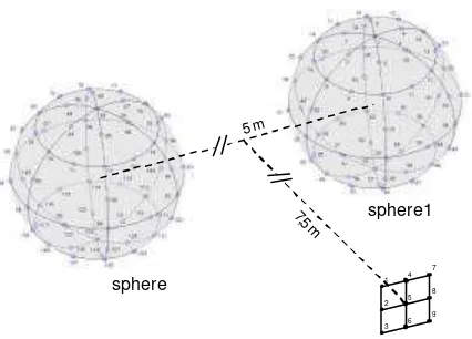
Figure 2. Configuration of sphere1, sphere2 and target field location (ο = node, = = field point)

Some test cases were done using numerical simulation for verifying the localization method of dominant surface area of multiple acoustic sources. The sources that are used in simulation consist of two spherical shape sources with radius a = 1 meter each. The surface of each source was discretized into 24 elements and 62 nodes as shown in Figure 2. The sphere1 source has node number 1 to 62 and the sphere2 source has node number 63 to 124. The simulations were done by first reconstructing the source surface acoustic parameter based on acoustic pressure data on the field points with a distance of 0.1 meter from the source surface. Then, find the acoustic transfer matrix for 9 target field points which are located on y-plane = 7.5 meter in Cartesian coordinate (Table 1).

1

6 4

9 8 7

3

2 5

7,5 m

5 m

sphere1

[image:4.596.317.530.285.438.2]

[image:5.596.323.514.119.350.2]

Table 1. Coordinate of target field points

FP x y z FP x y z FP x y z

1 2.3 7.5 0.2 4 2.5 7.5 0.2 7 2.7 7.5 0.2

2 2.3 7.5 0.0 5 2.5 7.5 0.0 8 2.7 7.5 0.0

3

2.3 7.5

-0.2 6 _2.5 7.5

-0.2 9 _2.7 7.5

-0.2

The first test case is the sphere1 source vibrates uniformly, while sphere2 source does not vibrate. The distance between sphere1 and sphere2 is 5 meter. The pressure magnitude on the surface of sphere1, sphere2, and on the target field location can be seen on Figure 3. Table 2 shows 9 of 124 nodes that are the most influential to each target field point for the first case.

[image:5.596.88.304.335.473.2]

Figure 3. Acoustic pressure magnitude on the surface of sphere1, sphere2, and target field points (case 1)

Table 2. The most influential nine nodes to each field point (FP) (case 1)

FP1 FP2 FP3 FP4 FP5 FP6 FP7 FP8 FP9

29 29 29 29 29 29 29 29 29

21 39 39 21 39 39 21 39 39

39 21 21 39 21 21 39 21 21

27 27 27 27 27 27 27 27 27

22 22 40 22 22 40 22 22 40

40 40 22 40 40 22 40 40 22

11 47 47 11 47 47 11 47 47

47 11 11 47 11 11 47 11 11

31 31 31 31 31 31 9 31 45

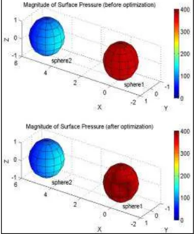
Figure 4. Acoustic pressure magnitude on the surface of sphere1, sphere2, before and after optimization (case 1)

The average of magnitude pressure on the target field points is 35.84 - 36.11i. If the average of desired or predetermined sound level (pressure) is 32.25 - 32.50i (decreased 10 %), then nodes that their pressure must be changed are node 29, 39, 21, 27, 22, 40, 47, 11, and 31. By using the developed inverse technique and optimization method, reconstruction of optimal surface acoustic pressure of multiple sources that fulfill the desired sound level on the target field points can be obtained. The reconstruction result can be seen in Figure 4 and the target field pressure that resulted from the optimized source characteristic can be seen in Table 3.

[image:5.596.94.288.558.692.2]

[image:6.596.84.300.152.322.2]

Tabel 3. Acoustic pressure on target field points (case 1)

Field Point

Resulted Pressure Desired Pressure

Real Im Real Im

1 32.16 -32.74 32.25 -32.50

2 32.37 -32.58 32.25 -32.50

3 32.16 -32.74 32.25 -32.50

4 32.11 -32.13 32.25 -32.50

5 32.31 -31.97 32.25 -32.50

6 32.11 -32.13 32.25 -32.50

7 32.30 -32.77 32.25 -32.50

8 32.50 -32.61 32.25 -32.50

9 32.30 -32.77 32.25 -32.50

The second test case, both sources vibrate non-uniformly. Sphere1 and sphere2 source vibrates with different surface normal velocity. The distance between sphere1 and sphere2 is 5 meter. The pressure magnitude on the surface of sphere1, sphere2, and on the target field location can be seen on Figure 5.

Figure 5. Acoustic pressure magnitude on the surface of sphere1, sphere2, and target field points (case 2)

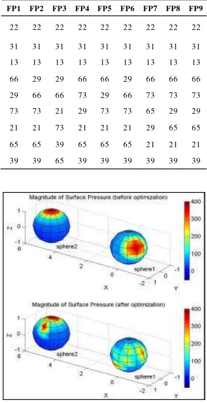
Table 4 shows 9 of 124 nodes that the most influential to each target field point for the second case. The average of magnitude pressure on the target field points is 3.33 - 18.33i. If the average of desired or predetermined sound level (pressure) is 2.83 - 15.58i (decreased 15 %), then nodes that their pressure must be changed are node 22, 31, 13, 66, 29, 73, 21, 65, and 39.

[image:6.596.316.520.262.659.2]

By using the developed inverse technique and optimization method, reconstruction of optimal surface acoustic pressure of multiple sources that fulfill the desired sound level on the target field points can be obtained. The reconstruction result can be seen in Figure 6 and the target field pressure that resulted from the optimized source characteristic can be seen in Table 5.

Table 4. The most influential nine nodes to each field point (FP) (case 2)

FP1 FP2 FP3 FP4 FP5 FP6 FP7 FP8 FP9

22 22 22 22 22 22 22 22 22

31 31 31 31 31 31 31 31 31

13 13 13 13 13 13 13 13 13

66 29 29 66 66 29 66 66 66

29 66 66 73 29 66 73 73 73

73 73 21 29 73 73 65 29 29

21 21 73 21 21 21 29 65 65

65 65 39 65 65 65 21 21 21

39 39 65 39 39 39 39 39 39

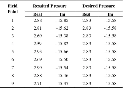
[image:6.596.88.300.429.561.2]

[image:7.596.85.300.151.304.2]

Tabel 5. Acoustic pressure on target field points (case 2)

Field Point

Resulted Pressure Desired Pressure

Real Im Real Im

1 2.88 -15.85 2.83 -15.58

2 2.81 -15.62 2.83 -15.58

3 2.69 -15.38 2.83 -15.58

4 2.99 -15.82 2.83 -15.58

5 2.93 -15.66 2.83 -15.58

6 2.69 -15.50 2.83 -15.58

7 2.99 -15.54 2.83 -15.58

8 2.88 -15.46 2.83 -15.58

9 2.71 -15.37 2.83 -15.58

From Table 5, it can be seen that the obtained characteristic of noise sources produce sound pressure level on the target field location that conform to the predetermined (desired) value. It means that the proposed method can be use for reconstruction an optimal surface acoustic parameter of multiple sources that fulfill the predetermined sound level on a certain target field location.

4. CONCLUSIONS

The reconstruction of multiple sources that fulfill the predetermined sound level on certain target field location has been presented in this paper. The proposed reconstruction method constitutes inverse and optimization methods that developed using Boundary Element Method and Conjugate Gradient. The sound level on the target field location that resulted from the sources that optimized by the proposed method is conform to the predetermined value. Optimization is sufficient done on the dominant surface area only.

REFERENCES

Bai, M.R., 1992. Application of BEM (Boundary Element Method) - Based Acoustic Holography to Radiation

Analy-sis of Sound Sources with Arbitrarily Shaped Geometries, J. Acoust. Soc. Am., vol. 92, 533-549.

Demmel, J.W., 1997. Applied Numerical Linear Algebra, University of California, SIAM Publishing Co.

Hansen, P.C.,1998 Rank-Deficient and Discrete Ill-Posed Problems, SIAM, Philadelphia. Ih, J.G. and B.K. Kim, 1998. On the Use of the

BEM-Based NAH for the Vibro-Acoustic Source Imaging on the Nonregular Exterior Surfaces, Proceedings of Noise-Con 98, Ypsilanti, Michigan, pp. 665-770. Kim, B.K. and J.G. Ih, 1996. On the

Reconstruction of the Vibro-Acoustic Field Over the Surface Enclosing an Interior Space Using the Boundary Element Method, J. Acoust. Soc. Am., vol. 100(5) , 3003-3016.

Kim, Y.K. and Y.H. Kim, 1999. Holographic Reconstruction of Active Sources and Surface Admittance in an Enclosure, J. Acoust. Soc. Am., 105(4), 2377-2383. Setiadikarunia, D., B. Soenarko, D Kurniadi,

dan Wono S. Budhi, 2006. Aplikasi Metoda Elemen Batas Untuk Menentukan Dominan Area Dari Sumber Akustik Terhadap Lokasi Medan Tertentu,

Prosiding Semiloka IV Teknolog i Simulasi dan Komputasi serta Aplikasi, - BPPT, Jakarta (2006), 84-91.

Setiadikarunia, D., 2007. Localization of Dominant Surface Area of Multiple Acoustic Sources, Proceedings of the 4th Ketingan Physics Forum, Solo.

Seybert, A.F., B. Soenarko, F.J. Rizzo and D.J. Shippy, 1985. An Advanced Computatio-nal Method for Radiation and Scattering of Acoustic Wave in Three Dimensions, J. Acoust. Soc. Am., vol. 77(2), 362-368. Soenarko, B., and D. Urika, 2005. An Inverse