Full Terms & Conditions of access and use can be found at
http://www.tandfonline.com/action/journalInformation?journalCode=ubes20
Download by: [Universitas Maritim Raja Ali Haji] Date: 11 January 2016, At: 22:29
Journal of Business & Economic Statistics
ISSN: 0735-0015 (Print) 1537-2707 (Online) Journal homepage: http://www.tandfonline.com/loi/ubes20
Flexible Approximation of Subjective Expectations
Using Probability Questions
Charles Bellemare , Luc Bissonnette & Sabine Kröger
To cite this article: Charles Bellemare , Luc Bissonnette & Sabine Kröger (2012) Flexible
Approximation of Subjective Expectations Using Probability Questions, Journal of Business & Economic Statistics, 30:1, 125-131, DOI: 10.1198/jbes.2011.09053
To link to this article: http://dx.doi.org/10.1198/jbes.2011.09053
View supplementary material
Published online: 06 Apr 2012.
Submit your article to this journal
Article views: 190
Flexible Approximation of Subjective
Expectations Using Probability Questions
Charles B
ELLEMAREDépartement d’Économique, Université Laval, Pavillon J.-A.-DeSève, 1025, avenue des Sciences-Humaines, Québec (Québec) G1V 0A6, Canada (cbellemare@ecn.ulaval.ca)
Luc B
ISSONNETTEDepartment of Econometrics and OR, Tilburg University, Warandelaan 2, PO Box 90153, 5000 LE Tilburg, The Netherlands (l.bissonnette@uvt.nl)
Sabine K
RÖGERDépartement d’Économique, Université Laval, Pavillon J.-A.-DeSève, 1025, avenue des Sciences-Humaines, Québec (Québec) G1V 0A6, Canada (skroger@ecn.ulaval.ca)
We propose a flexible method to approximate the subjective cumulative distribution function of an eco-nomic agent about the future realization of a continuous random variable. The method can closely ap-proximate a wide variety of distributions while maintaining weak assumptions on the shape of distribution functions. We show how moments and quantiles of general functions of the random variable can be com-puted analytically and/or numerically. We illustrate the method by revisiting the determinants of income expectations in the United States. A Monte Carlo analysis suggests that a quantile-based flexible approach can be used to successfully deal with censoring and possible rounding levels present in the data. Finally, our analysis suggests that the performance of our flexible approach matches that of a correctly specified parametric approach and is clearly better than that of a misspecified parametric approach.
KEY WORDS: Approximation of subjective probability distribution; Elicitation of probabilities; Spline interpolation.
1. INTRODUCTION
The measurement of subjective expectations has proven use-ful for eliciting knowledge of economic agents and experts on the future realization of various economic variables (e.g., Dominitz and Manski 1997; Engelberg, Manski, and Williams 2009) and improving the empirical content of stochastic models of choice under uncertainty (Bellemare, Kröger, and van Soest 2008; Delavande 2008). It has been advocated that the measure-ment of expectations should proceed by first measuring sub-jective probability distributions. In particular, there is growing evidence that agents reveal different points of their subjective distribution (mean, median, or other quantiles) when asked for their best point prediction of a future event (see Manski 2004 for a review). Thus, deriving expectations from probability dis-tributions can improve interpersonal comparisons while provid-ing more information on the uncertainty faced by respondents.
Up to now, two approaches have been used to make infer-ences on subjective distributions. The first approach is para-metric and assumes that the subjective distribution of a respon-dent is drawn from a parametric distribution (e.g., a normal or lognormal distribution) that depends on a finite number of un-known parameters. As with most parametric approaches, mis-specification of the underlying distribution may lead to biased forecasts and inferences. The second approach is fully nonpara-metric, placing no restriction of the nature or shape of subjec-tive distributions. This approach overcomes potentials biases due to misspecification of the underlying distribution at the ex-pense of providing set rather than point identification of the functionals of interest.
In this paper, we present a flexible method that yields point identification of the distribution function of a respondent while maintaining weak assumptions on the shape of the underlying distribution. The flexible approach builds on cubic spline in-terpolation, which requires only that the underlying distribu-tions be twice differentiable on their support. Moreover, the es-timation by cubic splines involves solving a system of linear equations. Thus our flexible approach provides a simple an-alytical solution for the estimated function. Cubic splines are well-known interpolation methods (see, e.g., Judd 1998); how-ever, to the best of our knowledge, they have not been applied to fit individual specific cumulative distribution functions using subjective expectations data. The closest work using interpola-tion methods to fit a cumulative distribuinterpola-tion funcinterpola-tion is that of Kriström (1990), who estimated the population-level distribu-tion of willingness to pay for an environmental good using lin-ear interpolation and aggregated survey responses to valuation questions.
We illustrate our approach by revisiting the determinants of expectations concerning future income using data from the Sur-vey of Economic Expectations (SEE). These data are character-ized by high levels of censoring and potential rounding. Censor-ing occurs when individuals report a nonzero probability that the future outcome will fall outside the range of potential val-ues spanned by the probability qval-uestions. The parametric ap-proach maintains sufficiently strong distributional assumptions
© 2012 American Statistical Association Journal of Business & Economic Statistics January 2012, Vol. 30, No. 1 DOI: 10.1198/jbes.2011.09053
125
126 Journal of Business & Economic Statistics, January 2012
to deal with censoring. In contrast, the flexible approach main-tains weaker distributional assumptions. As a result, estimated moments will be affected by censoring. To overcome this prob-lem, we propose a quantile-based flexible approach that uses the estimated median as a measure of central tendency and the estimated interquartile range (IQR) as a measure of respon-dent uncertainty. We compare estimators of the determinants of expectations and uncertainty using both a specific paramet-ric approach and our quantile-based flexible approach. We find that both approaches provide similar results for most determi-nants of future income, suggesting that the distributional as-sumptions chosen to implement the parametric approach are reasonable.
In the final part of the article, we present a Monte Carlo anal-ysis designed to measure the impact of censoring and rounding on estimates of the determinants of expectations. We focus on comparing the performance of our flexible approach with that of a correctly specified parametric approach as well as an in-correctly specified parametric approach. We find that the flexi-ble approach generates unbiased estimates of the determinants of expectations. This result holds when we introduce censoring and rounding levels believed to be present in the data. More-over, the performance of the flexible approach is comparable to that of the correctly specified parametric approach but clearly outperforms the incorrectly specified parametric approach that we consider.
2. A FLEXIBLE APPROACH
Our objective is to approximate the subjective probability distributionFi(z)=Pri(Z≤z)of a respondentiusing his or her
answers toJprobability questions of the type “what is the per-cent chance thatZis less than or equal tozj?,” wherez1<z2<
· · ·<zJ are threshold values. Thus theJ data points available
to make inferences onFi(z)are{(z1,Fi(z1)), . . . , (zJ,Fi(zJ))},
where 0≤Fi(zj)≤1 denotes the probability statement to a
question with thresholdzj. Censoring occurs whenFi(z1) >0 and/or 1−Fi(zJ) >0. This implies that some probability mass
is not contained within the interval[z1,zJ].
We propose to use the available data to approximate the sub-jective cumulative distribution functionFi(z)using cubic spline
interpolation. A cubic spline is a piecewise polynomial func-tion defined onJ−1 intervals,[z1,z2], . . . ,[zJ−1,zJ]. On each
interval, the functionFi(z)is assumed to be given by a
polyno-mialaj+bjz+cjz2+djz3, where(aj,bj,cj,dj)are the
interval-specific polynomial coefficients. The spline approximation of the functionFi(z)is constructed by simply connecting the
dif-ferent polynomials at the relevant threshold values. The set
{(aj,bj,cj,dj):j=1, . . . ,J−1}contains the 4(J−1)unknown
polynomial coefficients to be estimated. Exploiting continuity at the endpoints and interior thresholds provides 2J−2 equa-tions
Next, restrictions that the first and second derivatives ofFi(·)
agree at the interior thresholds generate 2J−4 additional equa-tions
bj+2cjzj+3djzj2=bj+1+2cj+1zj
+3dj+1z2j forj=2, . . . ,J−1,
2cj+6djzj=2cj+1+6dj+1zj forj=2, . . . ,J−1.
Two more conditions, so-called “boundary conditions” at the endpoints, are needed to estimate the 4(J−1)polynomial co-efficients of the cubic spline. There is very little guidance in the literature to chose these boundary conditions. Here we chose to impose thatF′′
i(z1)=Fi′′(zJ)=0, yielding what is known in
the literature as a natural cubic spline (see Judd 1998). Thus restrictions on the derivatives and the boundary conditions gen-erate a system of 4(J−1)linear equations that can be solved for the 4(J−1)unknown parameters. We experimented with boundary conditions restricting the first derivative at both end-points F′i(z1)=Fi′(zJ)=0 or by mixing restrictions on first
and second derivatives [e.g., setting F′′
i(z1)=F′i(zJ)=0 or
F′
i(z1)=F′′i(zJ)=0]. We found that these changes had only
minor effects on the estimated splines. We also experimented with linear and quadratic splines and found the cubic spline ap-proximation to be superior. We did not find that increasing the order of the spline further increased the quality of the approxi-mation. Thus, we use natural cubic splines throughout the rest of the article.
Absent censoring, moments can be directly estimated from the fitted subjective cumulative distribution function. In partic-ular, theλth noncentral moment ofZcan be computed analyti-cally using
h(·)is slightly more complicated. In such cases, numerical in-tegration can be performed by quadrature or simulation using
Fi(z). Similarly, quantiles can be obtained numerically by
in-vertingFi(z). Quantiles are especially useful in the presence
of censoring, which occurs when survey respondents report a nonzero probability thatZ will fall belowz1 and/or abovezJ.
In such cases, relevant medians can be used as a measure of central tendency, and the interquartile range (IQR) can be com-puted as a measure of subjective uncertainty as long asFi(z1) and 1−Fi(zJ)are less than or equal to 0.25.
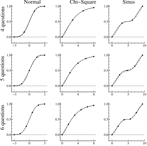
We illustrate the flexible approach by fitting three different distributions: a symmetric standard normal, an asymmetric chi-squared distribution with 3 degrees of freedom, and a bimodal distribution (with modes atπ/2 and 5π/2). The density of the bimodal distribution is given by sin(zA)+1 over the [0,3π] inter-val, whereA=2+3πensures that the function integrates to 1 over its domain. We fitted each cumulative distribution func-tion using between four and six data points equally spaced be-tween 3 and−3 for the normal distribution, between 0 and 8 for the chi-squared distribution, and between 0 and 3π for the bimodal distribution. The results are reported in Figure 1. As expected, the goodness of fit increases with the number of data points for all three interpolations. A slight approximation error
Figure 1. Fitted normal, chi-squared, and sinus distributions using cubic spline interpolations with four to six data points (questions). The solid lines represent the true distributions. The dashed lines represent the fitted distributions using the data points (dark points).
remains in the lower hand of the distribution when the number of data points is increased from four to six. Finally, we find that the approach has more difficulty fitting the bimodal distribution than the other two distributions. In contrast, the interpolation manages to provide a very good fit of the distribution with five or more data points.
Monotonicity
Cubic spline interpolation can produce oscillations that can cause the estimated distribution function to be nonmonotoni-cally increasing. This is particularly problematic when estimat-ing quantiles by invertestimat-ingFi(·)to obtain a unique solution.
Per-haps the simplest and most effective way to correct for these oscillations is to use the Hyman filter (Hyman 1983). This filter works in two steps. In a first step, definef′
i(zj)as the estimated
value of the first derivative of the spline function at the thresh-oldzj. Next, defineSi−1/2=(Fi(zj)−Fi(zj−1))/(zj−zj−1)and
Si+1/2=(Fi(zj+1)−Fi(zj))/(zj+1−zj) as the left-side slope
connecting with the previous threshold, (Fi(zj−1),zj−1), and the right-side slope connecting with the threshold (Fi(zj+1),zj+1). de Boor and Swartz (1977) have shown that if an estimated function satisfies the criteria
0≤fi′(zj)≤3 minSi−1/2,Si+1/2 , (2) then it is monotone on the interval[zj,zj+1]. Thus the criteria (2) can be used to identify all points where the monotonicity con-dition is violated. In a second step, the concon-dition of the equality of the second derivatives at each of the thresholds where mono-tonicity is violated is replaced by
fi′(zj)=minmax(0,fi′(zj)),3 minSi−1/2,Si+1/2 .
Hyman (1983) compared his filter approach to correct for nonmonotonicity with various alternative spline methods (e.g., Akima splines) and found that cubic spline interpolation cou-pled with his filter is the most effective method (in a mean squared error sense) to impose monotonicity on an estimated function.
3. REVISITING EXPECTATIONS OF FUTURE INCOME
In this section we illustrate the flexible approach by revisit-ing data on income expectations that were previously analyzed in a parametric setting by Dominitz (2001). Data are taken from the 1994–1995 SEE administered through WISCON, a national telephone survey conducted by the University of Wisconsin Survey Center. We focus on the following survey question:
What do you think is the percent chance (or chances out of 100) that your own total income, before taxes, will be under $zj(in the next 12 months)?
For each respondent, four initial thresholds zj were selected
based on self-reported minimal and maximal values for their income support. Respondents could then be asked one or two additional questions based on their four answers. A detailed de-scription of the branching algorithm to determine the income level or additional questions was presented by Dominitz (2001). We observe between four and six data points for each of 1249 respondents in the SEE aged 25–59 who were active in the la-bor force at the time they answered the SEE and who provided all of the information for our analysis.
Figure 2 documents the extent of censoring in these data by plotting the sample distributions ofFi(z1,i)andFi(zJ,i). We find
that only 44% of respondents have uncensored distributions at the lower end [Fi(z1,i)=0 in the left panel], whereas 66% of
respondents have uncensored distributions at the upper hand [Fi(zJ,i)=1 in the right panel]. Only 37% of all sample
respon-dents have uncensored distributions at both ends, a proportion too low to perform meaningful inferences using predicted mo-ments. We deal with censoring by using the median as the mea-sure of central tendency and the IQR as the meamea-sure of disper-sion. Note that a small subsample of respondents haveFi(z1,i)
or 1−Fi(zJ,i)exceeding 0.25 and (to a lesser extent) exceeding
0.5; thus the estimated medians and/or IQR of respondents in this subsample are potentially biased. We report a Monte Carlo analysis to assess how such biases affect the measurement of the determinants of expectations.
We compared estimates using our proposed quantile-based flexible approach with those of a parametric approach applied to the same data. The parametric approach involves fitting the best lognormal distribution when sufficient data points are available. Respondents who state at most one value ofFi(zj,i)that differs
from 0 or 1 are fitted with the bestlog-triangulardistribution, following the procedure of Engelberg, Manski, and Williams (2009).
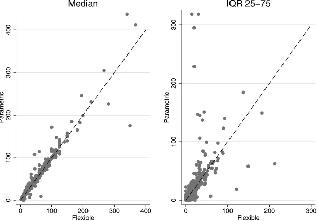
We applied the Hyman filter for 850 respondents (68%) to correct for nonmonotonicity of the cumulative distribution function predicted by the flexible approach. Figure 3 presents a scatterplot of the predicted medians (left panel) and IQR (right panel) using both approaches (the flexible on the horizontal axis and the parametric on the vertical axis). We found similar pre-dicted medians for both approaches, with predictions scattering
128 Journal of Business & Economic Statistics, January 2012
Figure 2. Distribution ofFi(z1,i)(left) andFi(zJ,i)(right) in the SEE data (N=1249). Dashed lines are at 0.25 (left) and 0.75 (right).
closely and relatively equally below and above the 45-degree line. More important differences emerge when looking at the predicted IQR. There the flexible method tends to predict higher dispersions (74.5% of predicted IQR are below the 45-degree line).
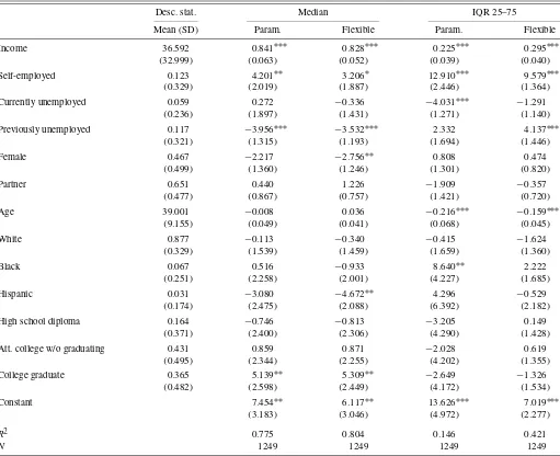
We next estimated linear models for both approaches using the predicted medians and IQR as dependent variables and us-ing a set of independent variables includus-ing realized income in the last year, basic demographic characteristics, employment status, and education level (using no high school diploma as the reference class). The first column of Table 1 presents some sample descriptive statistics of these variables. We estimated our models using the ordinary least squares (OLS) estimator with robust standard errors. Results are presented in subsequent columns of Table 1.
Overall, inferences using the flexible and parametric ap-proaches are similar, suggesting that the assumption of ex-pected income following a lognormal distribution is reasonable. Only small differences emerge. For instance, the flexible ap-proach predicts that women and Hispanics expect significantly lower average median future income. Both methods yield dif-ferent results concerning the effect of unemployment on the un-certainty of future income and the income unun-certainty faced by African-Americans. Results of the parametric approach suggest that the currently unemployed face significantly lower income uncertainty, whereas results of the flexible approach indicate that the previously unemployed have significantly higher in-come uncertainty. The parametric approach finds that African-American respondents have significantly greater income uncer-tainty, whereas this effect is smaller and insignificant using the flexible approach.
Figure 3. Scatterplot of estimated medians (left) and IQRs (right) of subjective income expectations, with either the parametric (vertical axis) or flexible (horizontal axis) method (N=1249). The dashed line represents the 45-degree line.
Table 1. Determinants of subjective medians and IQR in the SEE using the parametric and flexible approaches
Desc. stat. Median IQR 25–75
Mean (SD) Param. Flexible Param. Flexible
Income 36.592 0.841∗∗∗ 0.828∗∗∗ 0.225∗∗∗ 0.295∗∗∗
(32.999) (0.063) (0.052) (0.039) (0.040)
Self-employed 0.123 4.201∗∗ 3.206∗ 12.910∗∗∗ 9.579∗∗∗
(0.329) (2.019) (1.887) (2.446) (1.364)
Currently unemployed 0.059 0.272 −0.336 −4.031∗∗∗ −1.291
(0.236) (1.897) (1.431) (1.271) (1.140)
Previously unemployed 0.117 −3.956∗∗∗ −3.532∗∗∗ 2.332 4.137∗∗∗
(0.321) (1.315) (1.193) (1.694) (1.446)
Female 0.467 −2.217 −2.756∗∗ 0.808 0.474
(0.499) (1.360) (1.246) (1.301) (0.820)
Partner 0.651 0.440 1.226 −1.909 −0.357
(0.477) (0.867) (0.757) (1.421) (0.720)
Age 39.001 −0.008 0.036 −0.216∗∗∗ −0.159∗∗∗
(9.155) (0.049) (0.041) (0.068) (0.045)
White 0.877 −0.113 −0.340 −0.415 −1.624
(0.329) (1.539) (1.459) (1.659) (1.360)
Black 0.067 0.516 −0.933 8.640∗∗ 2.222
(0.251) (2.258) (2.001) (4.227) (1.685)
Hispanic 0.031 −3.080 −4.672∗∗ 4.296 −0.529
(0.174) (2.475) (2.088) (6.392) (2.182)
High school diploma 0.164 −0.746 −0.813 −3.205 0.149
(0.371) (2.400) (2.306) (4.290) (1.428)
Att. college w/o graduating 0.431 0.859 0.871 −2.028 0.619
(0.495) (2.344) (2.255) (4.202) (1.355)
College graduate 0.365 5.139∗∗ 5.309∗∗ −2.649 −1.326
(0.482) (2.598) (2.449) (4.172) (1.534)
Constant 7.454∗∗ 6.117∗∗ 13.626∗∗∗ 7.019∗∗∗
(3.183) (3.046) (4.972) (2.277)
R2 0.775 0.804 0.146 0.421
N 1249 1249 1249 1249
NOTE: Standard errors are in parentheses (Eicker–White used in OLS estimation). * Significant at 10% level. ** Significant at 5% level. *** Significant at 1% level.
3.1 Monte Carlo Analysis
We conducted a Monte Carlo analysis to assess how censor-ing and possible roundcensor-ing in the SEE income data can affect the results in our application. Our analysis focuses on compar-ing the performance of our proposed flexible approach with the performance of the parametric approach, using both correctly specified and misspecified distribution functions for the para-metric approach. We begin by specifying the data-generating process of medians mediand interquartile ranges IQRi
medi=θ0+θ1x1i+εi, (3)
IQRi=γ0+γ1x2i+ηi, (4)
where x1i and x2i are two determinants, and where εi and
ηi denote homoscedastic unobserved heterogeneity. Our
ob-jective is to analyze the properties of the OLS estimator of
(θ0, θ1, γ0, γ1)′ in the presence of censoring and rounding. To proceed, we specify (3) and (4) as equations generating quan-tiles of a Kumaraswamy distribution defined over the [0,1] in-terval with parameters(αi≥0, βi≥0). The Kumaraswamy
dis-tribution is sufficiently flexible to accommodate a wide range
of symmetric and asymmetric distributions of potential out-comes (Kumaraswamy 1980). For example, (αi=2, βi =2)
implies a symmetric distribution centered at 0.5, whereas(αi=
1, βi =5) produces a severely left-skewed distribution with
mode at 0.2. We specify our data-generating process in the following way. First, values of x1i and x2i are drawn from a
uniform distribution on the [−0.5,0.5] interval, whereas val-ues ofεi andηiare each drawn from a standard normal
distri-bution with mean 0 truncated to the [−0.1,0.1] interval. Fi-nally, we set (θ0=0.5, θ1=0.3, γ0=0.5, γ1=0.3). These data-generating processes force both medi and IQRi to lie
within [0.25,0.75]. We next present in detail the steps per-formed in our Monte Carlo simulations. Our analysis of the flexible and parametric approaches differs only with respect to step 4.
Step 1. Draw (medi,IQRi)for i=1,2, . . . ,N using
equa-tions (3) and (4).
Step 2. Compute for each i the parameters (αi, βi)
corre-sponding Kumaraswamy distribution by numerically solving
130 Journal of Business & Economic Statistics, January 2012
the following system of equations:
medi=Q0.5(αi, βi), (5)
IQRi=Q0.75(αi, βi)−Q0.25(αi, βi) (6)
such thatQκ(αi, βi)=F−1(κ;αi, βi)whereF−1(·)denotes the
inverse mapping of the Kumaraswamy cumulative distribution function F(x)=1−(1−xαi)βi evaluated at 0≤κ≤1 with
parameters(αi, βi).
Step 3.Generate points{zj,i:j=2, . . . ,J−1}using a
branch-ing algorithm inspired by our empirical application. In par-ticular, respondents with medi ≤0.42 are assigned the
vec-tor of thresholds (0,0.125,0.25,0.4,0.7,1), those with 0.42<
medi <0.59 are assigned thresholds (0,0.2,0.4,0.6,0.8,1),
and those with medi≥0.59 are assigned thresholds (0,0.3,0.6,
0.75,0.875,1). As with our empirical application, this algo-rithm assumes that prior information about the location of the distribution is used to generate thresholds. Then the cumulative probabilitiesF(zj,i;αi, βi)are computed at allzj,ivalues.
Step 4 (Flexible approach). Compute estimates medi and
IQRiusing the flexible approach.
Step 4(Parametric approach). Compute the value of δthat
minimizes the following loss function:
δ=arg min δ
(Pr(Z≤zj,i;δ)−Fi(zj,i,r))2,
where the summation is over the data points of respondent i
and Pr(Z≤zj,i;δ)denotes a parametric cumulative distribution
function with an unknown vector of parametersδ. We consider
the correctly specified case where Pr(Z≤zj,i;δ) is correctly
chosen to be the Kumaraswamy distribution with parameters
δ= [αi, βi]. We also consider a misspecified case where Pr(Y≤
zj,i;δ)is chosen to be the Normal distribution with meanτiand
varianceγi2. We compute estimatesmediandIQRiusingδ.
Step 5.Estimate the following equations:
medi=θ0+θ1xi+εi, (7)
IQRi=γ0+γ1xi+ηi, (8)
whereεi=εi+medi−mediandηi=ηi+IQRi−IQRi.
Equa-tions (7) and (8) are identical to equaEqua-tions (3) and (4), except that the true medians and IQRs are replaced by approximated
values generated using either the parametric approach or the flexible approach. Estimated values(θ0,θ1)′ and(γ0,γ1)′ are saved. We repeat steps 1–5 to for 10,000 samples of size 100.
The foregoing five steps generate our baseline results with-out censoring or rounding. To analyze the effects of rounding, we replace the probabilitiesF(zj;αi, βi)in step 3 by the closest
of the following numbers: 0, 1, 2, 3, 5, 10, 15, 20, 25, 30, 35, 40, 50, 60, 65, 70, 75, 80, 85, 90, 95, 97, 98, 99, or 100. This sequence closely matches the probability responses in our ap-plication. It also is one of the main rounding patterns discussed in the literature (see Manski and Molinari 2010).
To analyze the effects of censoring, we randomly draw for each ia pair of censoring levels from below and from above using the empirical distribution of censoring levels presented in Figure 2. Let c0
i andc1i denote these censoring levels. We
then rescale the thresholds assigned in step 3 such thatz1,i=
Qc0
i(αi, βi)andzJ,i=Q1−c1i(αi, βi).
We evaluate the performance of the flexible and parametric approaches with rounding and censoring by computing param-eter and standard error biases. Paramparam-eter bias is computed us-ing(1SSs=1φs−φ)/φ, whereφ∈ {θ0, θ1, γ0, γ1}are the true values and φs denotes the estimated parameter in simulation
s≤S=10,000. We also compute the percent bias of the esti-mated standard errors using(1SSs=1se(φs)−sd(φs))/sd(φs), where sd(φs)denotes the standard deviation of allφsand se(φs)
denotes the standard error predicted using the covariance ma-trix of the OLS estimator with homoscedasticity (σ2(X′X)−1). Thus we report the percent difference between the average dard error predicted by the OLS estimator and the actual stan-dard deviation of the estimates over the 10,000 simulations.
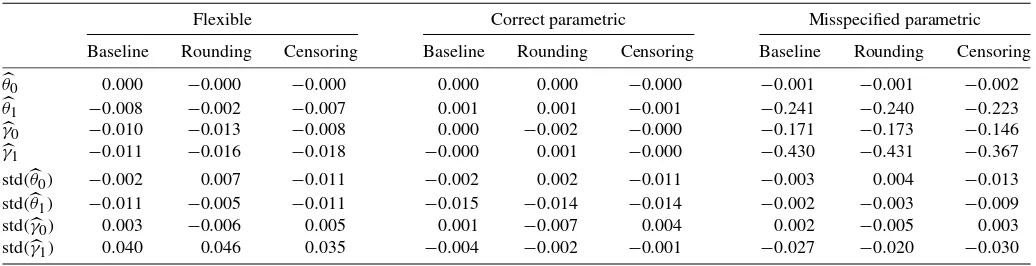
Table 2 presents the results. We see that under the baseline scenario (no censoring or rounding), both parameter and stan-dard error biases are small and negligible for the flexible and correctly specified parametric approaches. Of note, these re-sults also hold when censoring and rounding levels believed to be present in our data are incorporated in the analysis. This suggests that results of our empirical application are robust to censoring and possible rounding in the data. We also find that our flexible approach clearly outperforms the misspeci-fied parametric approach based on the erroneous assumption
Table 2. Lines(θ0,θ1,γ0,γ1)present the corresponding parameter biases computed using(1SSs=1φs−φ)/φ, whereφ∈ {γ0, γ1, θ0, θ1}are
the true values andφsdenotes the estimated parameter in simulations≤S=10,000. Lines std(·)present the percent bias of the estimated standard errors of the corresponding estimated parameter using(1SSs=1se(φs)−sd(φs))/sd(φs),
where sd(φs)denotes the standard deviation of allφs, and where se(φs)denotes the standard error predicted using the covariance matrix of the OLS estimator with homoscedasticity (σ2(X′X)−1)
Flexible Correct parametric Misspecified parametric
Baseline Rounding Censoring Baseline Rounding Censoring Baseline Rounding Censoring
that distributions are normal in the population. There parame-ter bias is substantial:−24% forθ1,−17% forγ0, and−43% forγ1. These biases are not affected by censoring and round-ing.
4. CONCLUSION AND DISCUSSION
Our Monte Carlo analysis suggests that the quantile-based flexible approach is robust to levels of rounding discussed in the literature and can accommodate censoring levels present in our data. We found that the flexible approach is comparable to a (first-best) correctly specified parametric approach in terms of bias and efficiency. Moreover, it clearly outperforms the mis-specified parametric approach that we consider. We interpret these results as an indication that the flexible approach repre-sents a potentially useful alternative to the existing parametric approach when researchers have little prior knowledge of the shape of the underlying distributions.
The flexible approach has three limitations. First, it lacks a distribution theory which would allow one to make infer-ences on individual specific distribution functions. This limi-tation might not pose a significant problem in practice, given that research on subjective expectations has focused on making statistical inferences on the determinants on expectations rather than on individual distribution functions. A second limitation is that moments are biased in the presence of censoring. This is expected because the flexible approach maintains weak as-sumptions on the shape of the distribution, thereby preventing extrapolation outside of the support spanned by the probabil-ity questions. Finally, our quantile-based flexible approach can accommodate only moderate levels of censoring.
Greater levels of censoring can be dealt with in several ways. The first and simplest way is to drop observations with exces-sive censoring. Though simple, this approach may introduce selection biases if the observations dropped represent a non-random subset of observations. A second way is to revert back to the parametric approach and maintain stronger distributional assumptions. Although this would allow accounting for censor-ing in the data, adoptcensor-ing a fully parametric approach introduces possible specification biases. Our analysis suggests that such
biases can be sizeable. Finally, the survey design could be im-proved by designing probability questions to gather informa-tion on a larger range of possible outcomes. The flexible ap-proach could then be used to make inferences while maintain-ing weaker assumptions on the underlymaintain-ing distributions.
ACKNOWLEDGMENTS
The authors thank Arthur van Soest, participants at the ESA meetings in Nottingham and Tucson, two referees, an associate editor, and the editor for comments. Financial support was pro-vided by the FQRSC. An OX code with files implementing all the procedures discussed in this paper can be downloaded at
http:// www.ecn.ulaval.ca/ charles.bellemare/.
[Received February 2009. Revised April 2011.]
REFERENCES
Bellemare, C., Kröger, S., and van Soest, A. (2008), “Measuring Inequity Aver-sion in a Heterogeneous Population Using Experimental DeciAver-sions and Sub-jective Probabilities,”Econometrica, 76, 815–839. [125]
de Boor, C., and Swartz, B. (1977), “Piecewise Monotone Interpolation,” Jour-nal of Approximation Theory, 21 (4), 411–416. [127]
Delavande, A. (2008), “Pill, Patch or Shot? Subjective Expectations and Birth Control Choice,”International Economic Review, 49, 999–1042. [125] Dominitz, J. (2001), “Estimation of Income Expectations Models Using
Ex-pectations and Realization Data,”Journal of Econometrics, 102, 165–195. [127]
Dominitz, J., and Manski, C. F. (1997), “Using Expectations Data to Study Subjective Income Expectations,”Journal of the American Statistical Asso-ciation, 92, 855–867. [125]
Engelberg, J., Manski, C., and Williams, J. (2009), “Comparing the Point Pre-dictions and Subjective Probability Distributions of Professional Forecast-ers,”Journal of Business & Economic Statistics, 27, 30–41. [125,127] Hyman, J. M. (1983), “Accurate Monotonicity Preserving Cubic Interpolation,”
SIAM Journal on Scientific Computing, 4 (4), 645–654. [127]
Judd, K. L. (1998),Numerical Methods in Economics, Cambridge, MA: MIT Press. [125,126]
Kristrom, B. (1990), “A Non-Parametric Approach to the Estimation of Welfare Measures in Discrete Response Valuation Studies,”Land Economics, 66, 135–139. [125]
Kumaraswamy, P. (1980), “A Generalized Probability Density Function for Double-Bounded Random Processes,”Journal of Hydrology, 46, 79–88. [129]
Manski, C. F. (2004), “Measuring Expectations,”Econometrica, 72 (5), 1329– 1376. [125]
Manski, C. F., and Molinari, F. (2010), “Rounding Probabilistic Responses in Surveys,”Journal of Business & Economic Statistics, 28, 219–231. [130]