Full Terms & Conditions of access and use can be found at
http://www.tandfonline.com/action/journalInformation?journalCode=ubes20
Download by: [Universitas Maritim Raja Ali Haji] Date: 11 January 2016, At: 23:07
Journal of Business & Economic Statistics
ISSN: 0735-0015 (Print) 1537-2707 (Online) Journal homepage: http://www.tandfonline.com/loi/ubes20
Infinite Density at the Median and the Typical
Shape of Stock Return Distributions
Chirok Han, Jin Seo Cho & Peter C. B. Phillips
To cite this article: Chirok Han, Jin Seo Cho & Peter C. B. Phillips (2011) Infinite Density at the
Median and the Typical Shape of Stock Return Distributions, Journal of Business & Economic Statistics, 29:2, 282-294, DOI: 10.1198/jbes.2010.07327
To link to this article: http://dx.doi.org/10.1198/jbes.2010.07327
Published online: 01 Jan 2012.
Submit your article to this journal
Article views: 95
Infinite Density at the Median and the Typical
Shape of Stock Return Distributions
Chirok HAN
Department of Economics, Korea University, Anam-dong, Seongbuk-gu, Seoul, Korea, 136-701 (chirokhan@korea.ac.kr)
Jin Seo CHO
School of Economics, Yonsei University, 262 Seongsanno, Seodaemun-gu, Seoul, Korea, 120-749 (jinseocho@yonsei.ac.kr)
Peter C. B. PHILLIPS
Cowles Foundation for Research in Economics, Yale University, PO Box 208281, New Haven, CT 06520-8281; Department of Economics, University of Auckland, Owen G Glenn Building, 12 Grafton Road, Auckland, New Zealand; School of Social Sciences, University of Southampton, Southampton SO17 1BJ, U.K.; and School of Economics, Singapore Management University, 90 Stamford Road, Singapore 178903, Singapore
(peter.phillips@yale.edu)
Statistics are developed to test for the presence of an asymptotic discontinuity (or infinite density or peakedness) in a probability density at the median. The approach makes use of work by Knight (1998) onL1estimation asymptotics in conjunction with nonparametric kernel density estimation methods. The
size and power of the tests are assessed, and conditions under which the tests have good performance are explored in simulations. The new methods are applied to stock returns of leading companies across major U.S. industry groups. The results confirm the presence of infinite density at the median as a new significant empirical evidence for stock return distributions.
KEY WORDS: Asymptotic leptokurtosis; Infinite density at the median; Kernel density estimation; Least absolute deviations; Stylized facts.
1. INTRODUCTION
Identifying the distributional shape characteristics of eco-nomic variables is an important aspect of statistical description and the search for stylized facts about economic data. Knowl-edge of the appropriate distributional class including tail shape and peakedness can be particularly important in designing suit-able methods of inference, in forecasting, in risk analysis, and in decision making on financial investments. Early studies in empirical finance, such as the classic articles of Mandelbrot (1963) and Fama (1965), recognized these advantages and ac-cordingly sought to identify some stylized distributional fea-tures of asset returns (such as heavy tailedness) to assist in lay-ing a statistical foundation for methods of empirical finance. More recently, the importance of distributional shape, density estimation and forecasting was acknowledged in the manage-ment of financial risk, the measuremanage-ment of value at risk, and in financial market volatility (e.g., Gabaix et al.2003; Ibragimov 2007; Ibragimov and Walden2007).
In much statistical work, it is conventional to suppose that the variables of interest have finite density over their entire sup-port. It is also convenient to rely on normal density functions or modified versions based on mixtures of normals in fitting economic data and in diagnostic statistical analysis. However, the condition of a finite density may be restrictive in some sit-uations, particularly for asset return data, which are generally acknowledged to be highly peaked at the median return. More-over, imposing the condition of a finite density when it is false will have consequences for inference. For example, applying
goodness-of-fit tests, such as the Kolmogorov–Smirnov test, can easily lead to inappropriate conclusions when the relevant density functions are not finite over their domains.
Heavy tailedness in returns is often accompanied by heavy concentrations of observations around the median return, which is commonly zero. This peakedness or leptokurtosis in the dis-tribution is a stylized fact for most financial asset return data. Sometimes the concentration around the median return may be so great as to produce an asymptote in the density at the me-dian. This “asymptotic leptokurtosis” is one focus of interest in the present article.
Existence of an infinite pole in the density combined with possible heavy tails is also important when evaluating various estimation techniques. In particular, the quality of least squares can be severely compromised if the error distribution has heavy tails, in which case least absolute deviation (LAD) estimation is an attractive alternative. As Knight (1998) pointed out, the finite sample and asymptotic properties of the LAD estimator are de-termined by how the density behaves around the median. When the density is infinite, then the LAD estimator is super consis-tent and it is, therefore, possible to construct sharper confidence intervals than the usual intervals that are based on least-squares estimation. However, assumptions relating to the existence of the density at the median were regarded as difficult to verify
© 2011American Statistical Association Journal of Business & Economic Statistics
April 2011, Vol. 29, No. 2 DOI:10.1198/jbes.2010.07327
282
(see Knight1998, p. 756) and no procedures for doing so have yet been suggested. The methodology proposed in the present article provides one solution to this issue.
The possible nonexistence of the probability density was re-cently considered by Zinde-Walsh (2008) from a different per-spective. By means of generalized functions and generalized random processes, Zinde-Walsh examined the asymptotic fea-tures of the kernel estimator for the conditional mean under general conditions. The present article differs in that we con-sider the median rather than the mean and also in that we di-rectly propose a method to test the existence of the density at the median.
Accordingly, the main theoretical goal of the article is to pro-vide a statistical test of infinite density at the median. Our ap-proach is to exploit the asymptotic theory of Knight (1998), and in particular, the mild regularity conditions under which the sample median is asymptotically normal when the density is finite and nonzero at the median. When the density has an in-finite discontinuity at the median, the sample median converges to the population median at a faster rate than the usual√nrate, wherenis the sample size. This simple differential provides a device for constructing test statistics for asymptotic leptokur-tosis that can be applied in general linear econometric models where there are other nuisance parameters to estimate. The ap-proach combines a nonparametric kernel density estimate at the median with the sample median to deliver a simple nonpara-metrically studentized test statistic.
The empirical goal of the article is to evaluate the leptokurto-sis of certain financial asset return data and assess the evidence in support of an infinite density at the median return. Much em-pirical literature already documents the nonnormality of asset return distributions and the leptokurtosis of these distributions (Mandelbrot1963; Fama1965). The present article takes the further step of testing for infinite density in stock returns. More specifically, we apply our tests to the return residuals from a simple autoregression. The empirical findings indicate that a significant number of leading companies in U.S. industries have asset returns with infinite density at the median. Accordingly, there appears to be evidence supporting infinite leptokurtosis as a new empirical evidence for some stock return distributions in the U.S.
The plan of the article is as follows. Section2develops the test statistic along with Monte Carlo experiments. Section 3 reports the empirical application and concluding remarks are given in Section4. Proofs and data information are given in the Appendix.
2. MEDIAN INFINITE DENSITY TESTS
We consider the linear regression model Y =Xβ +ε, whereYandXare n×1 and n×p matrices with of Yt and X′t, respectively, and ε=(ε1, . . . , εn)′. Our aim is in testing
whether or not the density ofεt is finite. For this purpose, we
first motivate the hypotheses and the test in the case of in-dependently and identically distributed (iid) disturbances and exogenous regressors. Then, the work is extended to the time series case allowing the regression errors to be conditionally heteroscedastic and the regressors to be predetermined (i.e., weakly exogenous). These extensions are important for our em-pirical application to financial data.
2.1 Motivational Remarks
We motivate our tests in a heuristic way by letting(X′ t, εt)be
iid, whereXtandεtare mutually independent. LetF(·)andf(·) be the cumulative distribution function (cdf) and the probabil-ity densprobabil-ity function (pdf) ofεt, respectively. It is well known
that the LAD estimator, sayβˆn, is√nconsistent and its asymp-totic distribution is√n(βˆn−β0)⇒(2f0)−1N(0,C−1)
when-ever f0:=f(0)is positive and finite under suitable regularity
conditions, whereC:=plimn−1X′X, and β0 is ap-vector of parameters defined asβ0:=argminβE|Yt−X′tβ|.
The meaning of the parameterβ0 is given in the literature in numerous ways. In regression contexts, β0 is identified by the zero conditional median assumption: median(εt|Xt)=0. If Xt =1, then β0 is itself the median of Yt, corresponding to
the 0.5th regression quantile of Bassett and Koenker (1978). Bloomfield and Steiger (1983), Pollard (1991), and Phillips (1991) also focused on quantile and/or LAD estimation and confirmed the result in various environments. Phillips (1991) worked under dynamic misspecification, Koenker and Zhao (1996) worked with the quantile regression model using time series data and conditionally heteroscedastic disturbances, and Kim and White (2003) studied a misspecified quantile regres-sion model with conditional heteroscedastic disturbances using iid data.
The situation is very different if f(x)asymptotes to infin-ity as x tends to zero. In that event, the convergence rate of the LAD estimator is determined by the divergence speed of
f(x)as x→0 and the shape of F(·) near zero. In such con-ditions, Knight (1998) developed LAD asymptotic theory for iid data under the condition that the sequence of functions
ψn(s):=√n[F(an−1s)−F(0)] converges to a nondegenerate
limit function. In this setting the scale componentan inψn(s)
is the convergence rate of the LAD estimator. For example, if
f(x)≃λα|x|α−1 nearx=0 for some α≤1 andλ∈(0,∞), then we have F(x)−F(0)≃λsgn(x)|x|α near zero, so that
ψn(s)→ λsgn(s)|s|α with an=n1/2α, as demonstrated by
Knight (1998). Thus, ifα=1 (sof0<∞),√n(βˆn−β0)has a
nondegenerate limit, whereas√n/an→0 and√n(βˆn−β0)= (√n/an)an(βˆn−β0)→p0 ifα <1 (sof0= ∞).
The present article exploits these differences in the limit be-havior of n1/2(βˆn−β0)under the different forms of f(x)in the vicinity of the origin to provide information about distrib-utional shape. A particular focus of attention relates to various leptokurtotic forms including extreme forms in which the den-sity asymptotes at the origin. The relevant hypotheses in this case can be formulated specifically in null and alternative forms as follows:
H0:f(0)∈(0,∞) versus H1:f(0)= ∞. (1)
The main motivation for considering these particular hy-potheses stems from empirical observations of financial data. As explained in theIntroduction, many financial asset returns exhibit distributions that appear so heavily peaked at the me-dian as to throw into doubt whether the density is finite at the origin. We seek to provide a mechanism for investigating this possibility in a formal manner with a statistical test procedure that enables a formal test of Equation (1).
If β0 were known, the goal of the present article could be relatively easily achieved by exploiting
ˆ
Bn:=4nˆf02(βˆn−β0)′C(βˆn−β0), (2)
as a suitable test statistic, whereˆf0is a density estimator forf0.
This quantity converges toχp2underH0, whereas underH1we have√n/an→0 andf0ˆ →p∞, so the limit behavior of
ˆ
Bn=4(√n/an)2
=o(1)
· ˆf02 =Op(1)
·a2n(βˆn−β0)′C(βˆn−β0)
=Op(1)
,
depends on how fast √n/an converges to zero and how fast
ˆ
f0diverges. In particular, if the divergence speed off0ˆ is slower than the convergence rate of√n/anto zero, then(√n/an)f0ˆ →p
0 and accordinglyBˆnconverges to zero in probability underH1.
As we discuss later more specifically, the Nadaraya–Watson es-timator based on the LAD residuals works well for this purpose as a density estimator if the bandwidth parameterδnconverges
to zero while√nδn→ ∞, i.e.,
δn+
1 √nδ
n→
0, asn→ ∞. (3)
The test statisticBˆn, therefore, enables a consistent test of H0
against H1 by exploiting the different asymptotic behavior of the statistic under the null and alternative. Specifically, we re-ject the null hypothesis at a given significance level if the test statistic is less than the corresponding left-tailed critical value of theχp2distribution. (The convergence ofBˆnto zero under the
alternative happens because the bandwidth is not too small. So one may suspect that a usual right-tailed test may be available if the bandwidth were chosen to converge to zero faster. But this strategy is not promising because then the accuracy offˆ0is so
poor that the test is considerably oversized.)
In practice,β0 is usually unknown, in which case, we can proceed by splitting the sample into two equal sized subsets. Ifnis even, equal sized subsets can be obtained by taking the first and second half of the sample. Ifnis odd, we may simply discard the first, the last, or the middle observation to obtain equal-sized subsets. If unequal subsets have to be used, the pro-cedures given in the following may be modified by rewriting in an obvious way analogous to the weighting used in the jack-knife (Quenouille1956).
Letβ˜1nandβ˜2n be the LAD estimators from the first sub-set (i.e., for t=1, . . . ,n/2) and the remainder of the sam-ple (i.e., t=n/2+1, . . . ,n), respectively. When X1 and X2 are the equal-sized submatrices of Xsuch thatX=(X′
1...X′2)′,
if n−1X′X→pC, then both (2/n)X′
1X1 and(2/n)X′2X2 also
converge to the same limit C, implying that for j =1,2, √n/
2(β˜jn −β0)⇒(2f0)−1C−1/2Zj under H0, where (Z1, Z2)′∼N(0,I). We may consider the differential√2nf0(β˜1n−
˜
β2n)as our test device, which weakly converges toC−1/2Z1− C−1/2Z
2 ∼ N(0,2C−1) under H0. Thus, it follows that nf02(β˜n)′C(β˜n)⇒χp2underH0, whereβ˜n:= ˜β1n− ˜β2n. Now a useful test statistic can be constructed from this quantity by replacingCandf0withn−1X′Xandf0ˆ, respectively. Again, the null distribution is χp2, whereas the statistic converges to zero in probability underH1. This heuristic explanation under-pinning the test can be formally stated as follows.
Theorem 1. Suppose that (Xt, εt)is iid overt, and that Xt
andεtare independent. Under AssumptionsAandBstated in
Section2.2withσt≡1, the following holds:
(i) Iff(0)∈(0,∞) andf(s)is continuous in a neighbor-hood of zero, thenBˆn⇒χp2.
(ii) Iff(0)= ∞, and Equation (10) in Section2.2holds, then ˆ
Bn→p0.
This theorem may be obtained as a special case of Theorem3 in the next section for conditionally heteroscedastic time series data (except that the covariance matrix of the LAD estimator is estimated under the iid and exogeneity assumption). We, there-fore, omit the proof and provide further discussion later.
2.2 Extensions to Time Series Contexts
The heuristic arguments that apply for iid data with strictly exogenous regressors can be extended to times series models with lagged dependent variables as regressors on the right-hand side and conditionally heteroscedastic errors. For this purpose, letFtbe the sigma field generated by(Xt, εt−1,Xt−1, εt−2, . . .)
and letεt:=σtet, whereσt is adapted toFt andet is iid with
pdffe(·). Our interest focuses on testing
H′
0:fe(0)∈(0,∞) versus H′1:fe(0)= ∞.
We also let Ft(s) and ft(s) denote the conditional cdf and
pdf ofεt, respectively, so that Ft(s)=P(εt≤s|Ft)=P(et≤ σt−1s|Ft)=Fe(σt−1s), andft(s):=Ft′(s)=σt−1fe(σt−1s).
Fur-ther, the previous definition of the quantityψn(s)is here
modi-fied toψnt(s)=√n[Ft(an−1s)−Ft(0)], whereanis selected so
thatψnt(s)has a nondegenerate (i.e., nonzero and finite) limit
on an open set. Ifft(0)is finite, thenan=√n, and ifft(0)= ∞,
then√n/an→0 by the same illustration of the power density
given above. Finally, we letnt(s):=0sψnt(r)drand also
de-noteft(0)asf0t for notational simplicity. Here, the functional nt(·)embodies the nonstochastic component of the centered
and rescaled objective functionZn(·)of Equation (4) below—
see also Equation (5). In the classical environment where there is a continuous error density, this term is further expanded to form the “denominator” of the asymptotic distribution of the LAD estimator as shown in Equation (6).
We allow for (σt) to be a stochastic process adapted to
Ft. Thus, the model can be interpreted within the frame-work of generalized autoregressive conditional heteroscedas-ticity (G)ARCH models (Bollerslev, Engle, and Nelson1994). The motivation for this setup follows from the fact that much economic data, particularly in finance, exhibit heteroscedastic behavior that is well characterized and frequently modeled in practice by the (G)ARCH effect. It is useful to employ the heteroscedasticity process(σt)in analyzing heavy-tailed
den-sities although this formulation is not identical to conventional (G)ARCH model effects unless conditional median and mean equations are the same.
We first establish LAD asymptotics by following Knight (1998, 1999). The argument is sketched here to exposit the main ideas and a formal statement is given in Theorem2, which is proved in Cho, Han, and Phillips (2010, hereafter CHP). The
asymptotic behavior of the LAD estimator is obtained by ana-lyzing the following rescaled and centered objective function:
Zn(u):=
where the second line follows from the representation|x−y| −
|x| = −ysgn(x)+20y[I(x≤s)−I(x≤0)]dsfor allx=0 (see Knight1998). BecauseZn(u)is minimized by the centred and
scaled estimator an(βˆn−β0), the behavior of an(βˆn−β0)
is determined by that of Zn(·). In particular, the minimizer an(βˆn−β0)ofZn(·)weakly converges to the minimizer of the
limit ofZn(·)under quite mild regularity conditions (e.g.,
As-sumptionA). Conveniently, it is sufficient to establish the point-wise probability limit ofZn(·)because it is a convex function
(see Knight1998and Geyer1996).
The limit of Zn(u) can be derived after obtaining the
lim-its of Zn(1)(u) and Zn(2)(u) separately. First, for the limit of Zn(1)(u), we simply apply a central limit theorem (CLT) for a
martingale difference array (MDA) under the usual regularity conditions, so thatZn(1)(u)⇒ −u′G, whereG∼N(0,C)with
The first term on the right-hand side is an average of an MDA, so that it should be negligible in probability, whereas the second term should follow a law of large numbers (LLN) under suitable regularity conditions. In particular, underH′
0we havean=√n
by the ergodic theorem because
nt(X′tu)=E[˜znt|Ft−1]
rem2details this argument more rigorously.
We again construct a more realistic test statistic for the un-known parameterβ0by splitting the sample into two subsets. Letβ˜1nandβ˜2n denote the two LAD estimates from the first
0. Finally, the unknown elementsCandAcan be
replaced by consistent estimators. As C is the limit variance of n−1/2nt=1Xtsgn(εt), it can be estimated consistently by
kernel functionK(·)and the bandwidthδnare required to
sat-isfy some regularity conditions, which are provided in Assump-tionBand in Theorem3. The feasible test statistic therefore has the following form
and as before the null hypothesis is rejected at a given signif-icance level if Bnis smaller than the corresponding left-tailed
critical value of theχp2distribution (e.g., 0.00393214 ifp=1 and the significance level is 5%).
We now examine the large sample behavior ofBn. We first
provide assumptions necessary for deriving the asymptotics of the LAD estimator. Given that εt=σtet, it is convenient and
common practice, though not strictly necessary here, to assume that et is iid. Further, the local behavior of the density around
zero is important for the asymptotics of the LAD estimator. Thus, we may assume that P(et≤s|Ft)=Fe(s)for all sin a
neighborhood of zero, which we calllocal homogeneity. Given this, if we let ψne(s):=√n[Fe(an−1s)−Fe(0)]and ne(x):=
The following assumptions are employed to establish the LAD asymptotics.
Assumption A. The following conditions hold:
(i) (X′
t, σt) is stationary and ergodic with σt2≥σ∗2>0,
such thatn−1nt=1σt2=Op(1)andEXt4<∞.
(ii) (et)is iid overt;etis independent of(X′t, σt)for eacht;
and for a functionh(·),|Fe(x)−Fe(0)| ≤h(x)for allx
in an open intervalV containing zero such thath(x) in-creases with respect to |x|, and for some finiteC0and n0, n1/2h(a−n1x)≤C0(1+ |x|) for all x∈R provided thatn>n0for somen0<∞.
(iii) For some ψe(·), there is a symmetric and nonneg-ative δ∗n(·) such that δ∗n(s) is increasing as |s| in-creases;|ψne(·)−ψe(·)| ≤δn∗(·), lim supn→∞E[Xt × δn∗(Xt)]<∞,δn∗(·) converges uniformly to zero on every compact neighborhood of zero.
(iv) E[sgn(et)|Ft] =0 andn−1/2max1≤t≤nXt →p0.
AssumptionAis almost identical to the conditions used in CHP to establish LAD asymptotics in an time series environ-ment that allows for conditional heterogeneity and weak ex-ogeneity. Some remarks on the conditions in Assumption A are in order. First, Assumption A(i) allows for the squared terms ofXt andεtto be correlated, so thatCmay not be
pro-portional to A,unlike Knight (1998). Second, the assumption that σt2≥σ∗2>0 implies that any heavy mass at zero is at-tributed to the density of et, not to the volatility process σt2.
Thus a median infinite density ofεt is sourced in and
equiva-lent to that ofet. Third, AssumptionA(ii) is satisfied by many
densities. For example, it is satisfied if fe(0) is finite or if
fe(x)=λα|x|α−1(i.e., the power density) forα <1 in a neigh-borhood of zero, so thatf(x)asymptotes to infinity asxtends to zero. Fourth, AssumptionA(iii) is provided to establish a limit property ofψne(·)in a way that its limit is a convex function. Finally, AssumptionA(iv) is useful for establishing a CLT for
n−1nt=1Xtsgn(εt). More detailed explanations on these
con-ditions can be found in CHP.
The following theorem presents the desired LAD asymptot-ics under these conditions.
Theorem 2(Cho, Han, and Phillips 2010). Given Assump-tionA,
an(βˆn−β0) ⇒ argmin
u∈Rp
(−u′G+τ (u)), (9)
where τ (u):=2 plimn−1nt=1t(X′tu), G∼N(0,C) with C:=plimn−1X′X.
This result from CHP (2010) develops the argument of Knight (1998, 1999) into a time series framework that suits the need of the current article. One difference between Theo-rem2 and the CHP result is that the CLT is directly assumed in CHP as a high level condition, whereas here it is derived by exploiting AssumptionA(iii). Theorem2 differs from Knight (1998, 1999) mainly because of the presence of conditional het-eroscedasticity. In our time series context,σtis not necessarily
constant, so that it leads to an information matrix inequality if
fe(0)is finite.
AssumptionAholds for many datasets and the power density illustrated previously is only one of many examples covered by
Theorem2. As in the iid data case, Equation (9) also implies that iffe(0) <∞, thenan=√nandτ (u)=u′Au, whereAwas
defined while obtaining the probability limit ofZ(n2)(u), thus
yielding the conventional result that√n(βˆn−β0)⇒12A−1G, whereas if fe(0)= ∞, then √n(βˆn− ˆβ0)=Op(a−n1√n)= op(1)asanis proportional tonγ withγ >1/2.
Next, we provide regularity conditions under which the test statisticBn defined previously has the desired asymptotic
be-havior under the null and alternative hypothesis on the error density. The conditions required mainly relate to the asymptotic behavior ofAˆndefined in Equation (7).
Assumption B. The following conditions hold:
(i) On a neighborhood of zero,fe(·) >0 andf¯e(y)/f¯e(x)≤
˜
Mfor some finiteM˜ for allxandyin the same neigh-borhood such that |x| ≤ |y|, where f¯e(x)= [Fe(x)− Fe(0)]/xforx=0.
(ii) The kernel functionK(·)satisfies:
(a) K(·) is a uniformly bounded nonnegative func-tion which is symmetric around zero and nonincreasing on the positive domain;
(b) K(x)dx=1,K(x)2dx<∞;
(c) for each y in a neighborhood of zero and for eachx,|K(x+y)−K(x)| ≤ ˙K(x)|y|, whereK(˙ ·)is uni-formly bounded and[sup|y|≥|x|K(y)˙ ]2dx<∞.
(iii) The bandwidth sequenceδnsatisfiesδn→0 andn1/2× δn→ ∞.
The Lipschitz condition in AssumptionB(ii)(c) is satisfied by many popular kernel functions. For example, if K(x)=
max(1− |x|,0), then the condition holds by letting K(x)˙ = I(−2≤x≤2)for|y| ≤1, whereI(·)is the indicator function. As another example, ifK(·)=φ (·)is the standard normal ker-nel, then for|y| ≤1, we can letK(x)˙ =sup|z|≤1{(x+z)φ (x+z)}
because K(x)˙ ≤φ (0)(|x| + 1)I(|x| ≤1)+(|x| +1)φ (|x| −
1)I(|x|>1), where the last bound is clearly square integrable. For the popular Epanechinikov kernelK(x)= {3/(4√5)}(1− 0.2x2)I(x2 ≤ 5), we can let K(x)˙ =0.3I(|x| ≤ 3). In gen-eral, if K(·) is differentiable, then AssumptionB(ii)(c) holds when|K′(·)|is uniformly bounded by a symmetric and square-integrable function which is nonincreasing on the positive do-main.
The limit behavior of the test statisticBnis given as follows.
Theorem 3. Under AssumptionsAandB, the following re-sults hold:
(i) Iffe(0)∈(0,∞)andfe(s)is continuous in a neighbor-hood of zero, thenBn⇒χp2.
(ii) Iff¯e(s)= [Fe(s)−Fe(0)]/sand ¯
fe(x)/f¯e(y)→ ∞ asx,y→0 andx/y→0, (10)
thenBn→p0.
Theorem3gives the limit behavior ofBnunder the null and
alternative hypotheses. A useful aspect of our testing proce-dure is that direct evaluation of et=σt−1εt is not required,
thus modeling the conditional variance process is not a nec-essary component of our test. Note that the condition in Equa-tion (10) is stronger than simply assuming thatfe(0)= ∞and
characterizes local behavior of fe(·) at the origin. This con-dition enables the test to discriminate null pdf’s from alter-natives. More specifically, this condition controls the diver-gence speed of fe(x) as x tends to zero. Even under the al-ternative of an infinite density, if the divergence speed is too slow then the discriminating information in finite samples of data may be too weak to identify the alternative. So, the con-dition in Equation (10) serves as a restriction in the class of alternative distributions that ensures test power against these alternatives. Many relevant density functions satisfy the condi-tion in Equacondi-tion (10) in spite of this restriction. As an exam-ple, for some c>0 and α <1 if Fe(x)∝1/2+csgn(x)|x|α
around zero, then¯fe(x)∝ |x|α−1, and therefore,f¯e(x)/f¯e(y)∝
|x/y|α−1, which diverges asx/y→0, so that Equation (10) fol-lows. A symmetrized gamma distribution with a shape parame-ter smaller than 1 also satisfies Equation (10). In general, the ra-tio[Fe(x)−Fe(0)]/[Fe(y)−Fe(0)] →0 under the alternative if
xapproaches zero faster thany. What Equation (10) further re-quires is that[Fe(x)−Fe(0)]/[Fe(y)−Fe(0)] →0 more slowly thanx/y→0, so that the ratio¯fe(x)/¯fe(y)diverges. An obvious counterexample to Equation (10) is a density with a logarithmic or other slowly varying discontinuities at the origin. For exam-ple, iff¯e(x)∼log(1/|x|)andy=x1−η for someη∈(0,1)as
x→0+,we have¯fe(x)/¯fe(y)→(1−η)−1asx→0+, thereby violating Equation (10). These density functions may not be discriminated from null densities by our test. So the test will not, in general, be powerful against densities with logarithmic type discontinuities at the median.
In simpler cases whereεt is independent ofXt, the testBn
can be further simplified. In such cases, we may use the sta-tisticB˜n:= ˜λ2n(β˜1n− ˜β2n)′(X′X)(β˜1n− ˜β2n)to test the same
hypothesis, whereλ˜nis defined by
˜
λn:=
1
n n
t=1
1
δn K
Yt−X′tβˆn δn
.
As before,B˜nweakly converges toχp2underH′0but converges
to zero underH′
1. The intuition behind this test is identical to
that underlying the generic test in Equation (2).
Before conducting Monte Carlo experiments for these tests, we remark that the limit distribution of the sample median de-pends on the local behavior of the probability density in the vicinity of the median and does not depend upon its behav-ior elsewhere, as shown by Knight (1998) and Rogers (2001). This property ensures that the limit distribution of statisticBˆn
also depends only on the shape characteristics of the probabil-ity densprobabil-ity near the median. Thus, asymmetry of the densprobabil-ity and possible discontinuities at points other than the median (e.g., at the mean if the mean and the median are different) do not affect the validity of the test.
2.3 Monte Carlo Experiments
We conduct a brief Monte Carlo experiment to examine the finite sample performance of the test. We use two data gen-erating processes (DGP’s) with autoregressive conditional het-eroscedasticity. Specifically, we suppose thatYt=0.4Yt−1+εt, εt=σtet, andσt2:=1+0.3ε2t−1, whereetis iid, and its density
function is (i) a two-sided gamma (double gamma) distribution
whose functional form is fe(x)= 12Ŵ(α)−1|x|α−1exp(−|x|)
and (ii) the mixtureαN(0,1)+(1−α)0. Accordingly,{εt,Ft}
is an MDA, and the conditional median equation is identical to the conditional mean equation, mainly due to the symmetry of the distribution of et. Further,fe(0)is finite when α=1 and
infinite whenα <1 for both DGP’s. Note that this DGP differs substantially from the usual case considered in the literature whereet is assumed to follow a standard normal distribution.
In practice, we generateetby lettinget=sgn(zt)vtfor DGP (i)
andet=zt{ut≥α}for DGP (ii), wherezt∼N(0,1),vtis
inde-pendently drawn from a gamma distribution with the “shape” parametersα, andut∼U(0,1). In our simulations, the
associ-ated random variables are generassoci-ated by thernorm,rgamma, andruniffunctions in R (R Development Core Team2008) and the LAD estimators are obtained by thequantreg pack-age in R (Koenker2008). The standard normal kernel is chosen for K(·), and the bandwidth parameterδn is set by the “rule
of thumb” parameter suggested by Scott (1992) as a variation of Silverman’s (1986) parameter, i.e., 1.06 times the minimum of the standard deviation and the interquartile range divided by 1.34 timesn−1/5. This bandwidth is popularly selected for em-pirical data analysis in the literature and is easy to compute. It is, therefore, of interest to see how this bandwidth performs in our experiments.
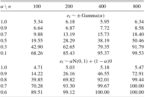
The simulation results are reported in Table1. The findings indicate that size (α=1)is approximately accurate, and power (α <1) approaches one as the sample size increases or theα pa-rameter gets smaller, which corresponds to sharper asymptotes in the density. (For both DGP’s the test seems slightly over-sized, but this disappears as the sample size further increases.) For the first DGP, power increases rather slowly whenαis close to unity as the sample size increases. This behavior is indicative of the inconsistency in the test that arises when Equation (10) fails. The second DGP is not regular ifα >0 because then the disturbance term has a discontinuous cdf at zero. Power behaves normally in this case as well.
Additional experiments were conducted. We first consid-ered an asymmetric conditional variance process similar to
Table 1. Simulation results for an AR(1)and ARCH(1)model from 10,000 iterations (5% level). DGP:yt=0.0+0.4yt−1+εt,
εt=σtet,σt2=1+0.3εt2−1. Bandwidth=1.06 min{SD,
(interquartile range)/1.34}n−1/5,K(·)=φ (·)
α\n 100 200 400 800
et∼ ±Gamma(α)
1.0 5.34 6.18 5.95 6.34
0.9 6.64 6.87 7.72 8.58
0.7 9.88 13.19 15.73 18.40
0.5 19.55 28.29 38.19 50.46
0.3 42.90 62.65 79.35 91.79
0.1 68.26 85.43 95.37 99.53
et∼αN(0,1)+(1−α)0
1.0 4.71 5.03 5.18 5.47
0.9 14.22 26.16 46.55 72.91
0.8 39.85 69.82 92.01 99.44
0.7 70.28 93.30 99.67 100.00 0.6 89.51 99.12 100.00 100.00
NOTE: α=1.0: size,α <1: power.
threshold-GARCH (TARCH), and obtained similar results which are omitted for brevity. Bandwidths selected by cross-validation were also examined, but the finite sample perfor-mance of the test in this case was found to be inferior to that of the test based on Scott’s rule of thumb. Issues of kernel and bandwidth choice obviously deserve further investigation in the present context. Based on the limit theory and the reported sim-ulations, we used the Gaussian kernel and Scott rule-of-thumb methods in our empirical applications.
3. EMPIRICAL APPLICATIONS
Asset return distributions are well known to exhibit non-normality. As overviewed in Bollerslev, Engle, and Nelson (1994), the early articles of Mandelbrot (1963) and Fama (1965) pointed out the leptokurtic feature of many asset re-turn distributions. Other stylized facts concerning asset rere-turns are the typical heavy tails of their distributions and the volatil-ity clustering manifested in squared returns, various realized volatility measures, and fitted (G)ARCH models.
The focus of the present study is to examine the leptokurto-sis of asset return distributions more carefully and test whether there is empirical support for “infinite leptokurtosis” arising from infinite density at the median. This section reports the re-sults of applying our tests to stock returns of leading companies in U.S. industries. More precisely, we apply our test in Equa-tion (8) to the autoregression
ri,t=αi,0+βi,0ri,t−1+εi,t, (11)
whereri,tis the return of theith company stock in periodt. The
companies used for our empirical applications are the so-called America top 400 large companies as announced byForbes.com
on December 22,2005. These companies are selected accord-ing to the Forbes.com criteria of helping investors to identify potential star stocks across 26 industries. In collecting this stock price data for the last 15 years (from May 24, 1991 to May 23, 1996) usingDatastream Advance 3.5, 242 companies are found to provide a full dataset with no missing observations. The com-panies are listed inAppendix Band the total number of obser-vations is 3799 after eliminating holiday obserobser-vations.
Time series features of daily returns are analyzed via Equa-tion (11), which attempts to capture any potential serial depen-dence in daily returns that may be induced from a variety of sources, including microstructure effects. Indeed, Equation (11) is often motivated as a reduced-form equation in the finance literature. For example, Lo and MacKinlay (1988, 1990), Sc-holes and Willams (1977), Dimson (1979), and Cohen et al. (1983a, 1983b) recognized that the betas in the standard capital asset pricing model (CAPM) cannot be consistently estimated by ordinary least squares (OLS) regression because of serially correlated residuals induced by nonsynchronous trading. Also, from a time series perspective, Nelson (1991) suggested that an autoregression be used to eliminate serial correlation. Ac-cordingly, we specify Equation (11) as a suitable reduced-form time series model for returns, without being specific about the underlying source of the weak dependence.
The disturbance termεi,tin Equation (11) is expected to
pos-sess time varying volatility features and to satisfy the MDA
condition. Note that the leptokurtosis feature of daily stock re-turns cannot be separated from the time varying volatility ef-fects, as pointed out by Bollerslev, Engle, and Nelson (1994). We explicitly allow for the presence of time varying volatil-ity in writingεi,t=σi,tei,t, whereei,t is iid, andσi,tis adapted
to Fi,t, which we define as the smallest σ-field generated by(ri,t−1,ri,t−2, . . .)for eachi=1,2, . . . ,242. Based on this
modeling framework, we test whether or not the density ofεi,t
is finite at zero. As detailed earlier,Bnis consistent even when
time varying volatility is part of the DGP, thereby enabling us to examine the leptokurtosis of financial asset returns in a context that accommodates this volatility.
The test is implemented using the following procedure. First, Equation (11) is estimated by both LAD and OLS regression methods, and we compare the prediction errors obtained from these. Note that OLS provides consistent estimates of the Equa-tion (11) when {εi,t,Fi,t}is an MDA having finite variance.
However, as remarked earlier, the limit of the LAD estimator may be different from OLS when the conditional mean and me-dian equations are different. Hence, we first check whether OLS estimation yields symmetric prediction error distributions. For this, we apply the runs test developed by McWilliams (1990) to our OLS residuals and test the following hypotheses:
H′′
0:fiv(·)is symmetric versus H′′1:fiv(·)is asymmetric,
wherefiv(·) is the pdf of vi,t, which is the OLS residual
ob-tained by estimating AR(1) model for each i. According to McWilliams (1990), the runs test is more powerful against a certain family of alternatives than other tests such as the Cramér–von Mises test constructed from the empirical bution. Also, the runs test does not assume a continuous distri-bution forvi,t, which is violated under the infinite density
hy-pothesis, so that symmetry of the pdf may not be properly tested by tests that rely on the empirical distribution. These properties give the runs test some potential advantages in the present con-text.
Next we apply the test in Equation (8) to the prediction errors obtained by LAD estimation of all companies and the compa-nies with symmetric densities according to the runs test. In par-ticular, we examine how the test statistics behave over subsam-ples with different sample sizes. Specifically, we start the data analysis by testing the hypotheses using the dataset with 1850 observations (February 2, 1999 to May 23, 2006) and comput-ingp-values. Then we perform the same testing procedure us-ing enlarged datasets with 2050 observations (April 17, 1998 to May 23, 2006). In this way we continue to increase the sample size and apply the test to multiple datasets growing in size by 200 observations each time until the sample size reaches 3799 (May 24, 1991 to May 23, 2006). The information from this sequence of tests is collected for each company, the number of companies rejecting the null is counted, and some collective conclusions are then deduced concerning the evidence in sup-port of infinite density.
The stated procedure is partly motivated by the fact that we reject the finite density hypothesis forBnclose to zero. Even
under the finite density hypothesis,Bn will still realize some
values close to zero with low probability. The above sequential testing procedure serves to raise the rejection probability and
increase test power for those companies that do exhibit infinite density at the median.
Due to space constraints, we do not attempt to report the analysis in full for all the companies considered in the study. Instead, we mainly focus on a specific industry—Health Care Equipment and Services (HCES)—for the presentation of de-tailed findings, as the results for this industry are fairly typical. Later in the discussion we provide some key summary results for all 242 companies and for those companies with symmetric densities according to the runs test.
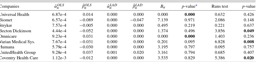
Table2compares the parameter estimates obtained by OLS and LAD estimation methods. For the nine companies in the HCES industry there are close similarities and some differences in the parameter estimates. The estimated intercepts are all very close to zero for both estimation methods. The fitted autoregres-sive (AR) coefficients are also small and the two estimates have the same signs in each case, but there are some small system-atic differences, most notably that the LAD estimates are all closer to zero than the corresponding OLS estimates. Neverthe-less, we cannot at the moment test whether or not the estimated LAD parameters converge to zero, as the asymptotic distribu-tion of thet-statistic for the LAD estimator critically depends on the assumption of finite density, which we want to test in the present article.
Table 2 also reports test statistic values and associated p -values (left-tailed) for the infinite density test. The outcomes differ according to the significance level. At the 5% level, for example, two companies (Universal Health and Omnicare) have infinite density at the median, and at the 1% level one company (Omnicare) has infinite density. This aspect is further accompa-nied by the runs test. At the 5% level, three companies (Becton Dickinson, Varian Medical System, and Coventry Health Care) have asymmetric densities, so that every company with infinite densities according to the statisticBnturn out to have
symmet-ric error densities. Overall, a significant number of companies seem to display strong empirical evidence in support of infinite density at the median in the HCES industry.
Extending this analysis to other industries, we collect the re-sults together in Tables3and4. First, we report the proportion of rejections of the null hypotheses of finite and symmetric den-sities in Table3. The columns of Table3contain the results of testing symmetry using the runs test based upon OLS residu-als, and the rows indicate the results of testing finite density us-ingBnwhen the level of the test is 5%. Thus, 40 companies turn
Table 3. Testing finite and symmetric densities at 5% level. Sample period: May 24, 1991 to May 23, 2006
Densities Symmetric Asymmetric Sum
Infinite 40 (21.39%) 17 (30.91%) 57 (23.55%) Finite 147 (78.61%) 38 (69.09%) 185 (76.45%)
Sum 187 (100.0%) 55 (100.0%) 242 (100.0%)
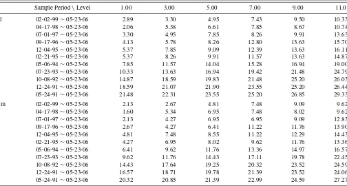
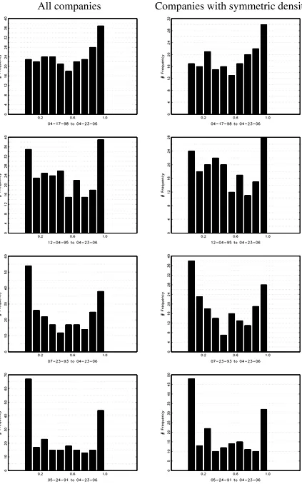
out to have infinite and symmetric densities, and this approxi-mately amounts to 21.39% of the companies with symmetric densities (16.53% of all companies). Next, we examine these findings in relation to the overall tendency to reject the null of finite density. Table4summarizes results for the full set of 242 companies (denoted by “All”) and its subset of 187 companies with symmetric error densities according to Table3(denoted by “Sym.”). The table provides the number of companies rejecting the null over different subsamples at various significance levels (1% to 11%). For example, if the level of the test is 5%, then 6.61% (resp. 6.95%) out of the 242 (resp. 187) companies reject the null when the sample period is April 17, 1998 to May 23, 2006. What we observe from Table4 is that the rejection rate for the finite density hypothesis gets larger as the number of observations gets bigger. This is observed not only for the 5% level of significance, but also for the other levels. This aspect is affirmed in Figure1, which shows the histograms ofp-values obtained for some of the sample periods in Table4. Evidently, morep-values cluster around zero as sample period gets larger for both groups of the companies.
This evidence taken together amounts to strong support of infinite density at the median as a remarkable new stylized dis-tributional feature for U.S. industry stock returns.
4. CONCLUDING REMARKS
This article develops and applies a new testing procedure to evaluate kurtosis and explicitly test whether a probability den-sity has an asymptote or infinite discontinuity at the median. The approach makes use of the limit theory forL1 estimation
pioneered by Knight (1998) and extended in recent work by the authors (CHP 2010), which allows for such discontinuities in the density in time series settings that include conditional het-erogeneity and serial dependence. The power of the test stems simply from the fact that the sample median converges to the
Table 2. OLS and LAD estimators and test statistic values. Sample period: May 24, 1991 to May 23, 2006
Companies αˆnOLS βˆnOLS αˆnLAD βˆLADn Bn p-value∗ Runs test p-value
Universal Health 6.87e–4 0.014 0.000 0.000 0.000 0.000 0.632 0.426
Biomet 6.57e–4 −0.089 0.000 −0.047 7.139 0.971 2.086 0.148
Stryker 7.57e–4 −0.005 0.000 0.000 0.495 0.219 0.221 0.637
Becton Dickinson 4.44e–4 −0.052 0.000 0.000 1.374 0.496 3.856 0.049
Omnicare 9.23e–4 0.031 0.000 0.000 0.000 0.000 1.403 0.236
Varian Medical Sys. 7.67e–4 −0.031 0.000 0.000 0.201 0.095 6.828 0.008
Humana 5.79e–4 −0.030 0.000 0.000 3.195 0.797 0.095 0.757
UnitedHealth Group 9.28e–4 0.037 0.001 0.020 3.161 0.794 0.685 0.407
Coventry Health Care 1.12e–3 −0.012 0.000 0.000 3.535 0.829 5.386 0.020
NOTE: ∗Left-tailedp-values.
Table 4. Proportion of rejected companies out of 242 companies (in percent). Model:ri,t=αi,0+βi,0ri,t−1+εi,t
Sample Period\Level 1.00 3.00 5.00 7.00 9.00 11.0
All 02-02-99∼05-23-06 2.89 3.30 4.95 7.43 9.50 10.33
true median at a rate faster than √n rate when the density is infinite at the median.
The test has some useful features for empirical applications. In particular, it is free from other nuisance parameters, does not rely on particular technical conditions such as differentiability or continuity of the underlying density function, is applicable to a wide class of densities, and can be used in a time series regression context.
Empirical application of the test to stock returns of lead-ing companies across U.S. industry is conclusive and provides strong evidence in support of infinite density at the median as a new significant empirical characteristic for stock return distri-butions. A significant number of the companies considered in the empirical analysis conducted here reject the null hypothe-sis of a finite density in favor of infinite density at the median. One implication of this finding is that data analysis in finan-cial econometrics that relies on distributions with finite density at the median, such astdistributions and mixtures of normals, will inevitably involve some distributional misspecification in the presence of infinite density.
APPENDIX A: PROOFS
Lemma 4. Let A˜n=n−1nt=1δn−1K(δ−n1εt)XtX′t. Ifn−1× n
t=1EXt3is uniformly bounded and√nδn→ ∞, then
un-der the conditions for Theorem2, we haveAˆn− ˜An→p0.
Proof. The proof is straightforward because
ˆAn− ˜An ≤1
expectation (first conditional onFt for each t and then aver-aging unconditionally), and noting thatnisop(1)because
n=(n1/2δn)−1√n(βˆn−β0).
Lemma 5. Suppose that the assumptions for Lemma4hold. Assume further thatfe(0) <∞,fe(s)is continuous in a
neigh-which is the average of an MDA. Its variance is bounded by
1
Figure 1. Histograms ofp-values (left-tailed). Model:ri,t=αi,0+βi,0ri,t−1+εi,t.
son−1nt=1E(Wnt|Ft)is integrable, and it converges to zero
Proof of Theorem3(i). Under the null, Lemmas4and5 im-ply that Aˆn− ˜A∗
n→p0. The result follows from Theorem 2
becauseA˜∗n→pA.
To handle the case under the alternative hypothesis, we need some technical lemmas. We start with the following.
Lemma 6. Under Assumption B(i) and (ii), if L(·)is con-tinuous, nonnegative and integrates to a strictly positive num-ber over√ (−∞,∞), then for n sufficiently large, 0<M0≤
Proof of Lemma6. We prove the result by considering in-tegration over the positive domain only as the negative do-main can be treated similarly. Define 0=b0≤b1≤b2≤ · · · bound,ψ (bk)is strictly positive for some finitekby
Assump-tionB(ii), implying that 12A∗n>0 for allnlarge enough.
Lemma 7. Given the assumptions for Theorems 2 and 3, if Equation (10) holds in addition, then for any uniformly bounded nonnegative functionL(·)which is symmetric around zero and nonincreasing over the positive domain, we have√
n an
L(x)fe(δnx)dx→0.
Proof. We show only that
A∗∗n = by virtue of the symmetry of L(·). Without loss of general-ity, we letL(0)=1 [otherwise, divide L(x) by L(0)]. Let m
Lemma6, and therefore,
A∗∗n =
Equation (A.1), and thereby complete the proof.
Lemma 8. Under Equation (10),(√n/an)Aˆn→p0.
APPENDIX B: LIST OF COMPANIES INCLUDED IN THE EMPIRICAL APPLICATION
The following lists the companies of each industry included for our empirical analysis. The number of companies is pro-vided in parentheses for each industry.
Aerospace & Defense (5): Goodrich, General Dynamics, Al-liant Techsystems, Moog, DRS Technologies.
Banking (13): Citigroup, Synovus Finl, Zions Bancorp., Wells Fargo, Popular, M&T Bank, AmSouth Bancorp., Mar-shall & Ilsley, Golden West Finl., Wachovia, Commerce Ban-corp., Bank of America, Compass Bancshares.
Business Services & Supplies (9): Automatic Data, Paychex, Avery Dennison, Robert Half Intl, Waste Management, Service-Master, Manpower, Equifax, World Fuel Services.
Capital Goods (12): Danaher, Valmont Inds., Ingersoll-Rand, Timken, Donaldson, Cummins, JLG Indst., Caterpillar, Ame-tek, Rockwell Automation, Genlyte Group, Oshkosh Truck.
Chemicals (10): Ecolab, Engelhard, Rohm and Haas, Dow Chemical, Airgas, Sigma-Aldrich, Air Prods & Chems, Valspar, Lubrizol, Georgia Gulf.
Conglomerates (6): General Electric, Dover, Emerson Elec-tric, Fortune Brands, United Technologies, ITT Inds.
Construction (9): Jacobs Engineering, Standard Pacific, Toll Brothers, Lennar, Pulte Homes, MDC Holdings, KB Home, Ry-land Group, Meritage Homes.
Consumer Durables (13): Harley-Davidson, Toyota Motor, Honda Motor, Nissan Motor, Volvo, Brunswick, Johnson Con-trols, Black & Decker, Genuine Parts, Applied Inds., Paccar, Toro, Thor Inds.
Diversified Financials (4): Charles Schwab, Berkshire Hath-away, Franklin Resources, Legg Mason.
Drugs & Biotech (5): Abbott Laboratories, Allergan, Amgen, Johnson & Johnson, Barr Pharmaceuticals.
Food Drink & Tobacco (12): Coca-Cola, General Mills, PepsiCo, Wm Wrigley Jr., Seaboard, PepsiAmericas, Mc-Cormick & Co, Hormel Foods, Kellogg, Dean Foods, Constel-lation Brands, Pilgrim’s Pride.
Food Markets (4): Sysco, Weis Markets, Ruddick, Casey’s General Store.
Health Care Equipment & Services (9): Universal Health, Biomet, Stryker, Coventry Health Care, Becton Dickinson, Om-nicare, Varian Medical Systems, Humana, UnitedHealth Group.
Hotels, Restaurants & Leisure (5): Brinker Intl., Hilton Ho-tels, Applebee’s Intl., MGM Mirage, Carnival Corp.
Household & Personal Products (8): Timberland, Procter & Gamble, Liz Claiborne, Oxford Indst., Alberto-Culver, NIKE, Church & Dwight, Phillips-Van Heusen.
Insurance (10): Chubb, Aflac, Cincinnati Finl., Old Republic Intl., Mercury General, White Mountains Ins., First American, Commerce Group Inc., Selective Ins., Zenith National Ins.
Materials (12): Barrick Gold, Bemis, Worthington Inds., Phelps Dodge, Inco, Harsco, Massey Energy, Nucor, Commer-cial Metals, Steel Technologies, Quanex, Cleveland-Cliffs.
Media (9): Comcast, Walt Disney, WPP Group, Omni-com Group, EW Scripps, Meredith, RR Donnelley & Sons, McGraw-Hill Cos., Banta.
Oil & Gas Operations (16): Nabors Industries, Baker Hughes, Noble Corp., Marathon Oil, Smith International, Ash-land, Apache, EOG Resources, Holly, BJ Services, Murphy Oil, Tesoro, Valero Energy, Sunoco, Western Gas Resources, Occi-dental Petroleum.
Retailing (17): CVS, Walgreen, Home Depot, Tiffany & Co., Dollar General, Genesco, Sherwin-Williams, Claire’s Stores, Lowe’s Cos., Fastenal, Staples, AutoNation, Best Buy, Williams-Sonoma, Ross Stores, Nordstrom, Michaels Stores.
Semiconductors (7): Intel, Maxim Integrated Prods, Altera, Linear Technology, Texas Instruments, KLA-Tencor, Lam Re-search.
Software & Services (6): Microsoft, Adobe Systems, Fiserv, Electronic Arts, CACI International, Autodesk.
Technology Hardware & Equipment (10): EMC, Cisco Sys-tems, Dell, Motorola, Benchmark Electronics, Canon, Harris, Western Digital, Harman Intl., Apple Computer.
Telecommunications Services (5): Verizon Commun., Bell-South, CenturyTel, Sprint Nextel, Alltel.
Transportation (8): Southwest Airlines, SkyWest, FedEx, CSX, Werner Enterprises, Expeditors Intl., Burlington Santa Fe, JB Hunt Transport.
Utilities (18): National Fuel Gas, Nicor, Constellation En-ergy, Laclede Group, OGE EnEn-ergy, Scana, MDU Resources, New Jersey Resources, Exelon, AGL Resources, FirstEnergy, Edison Intl., Sempra Energy, Wisconsin Energy, WPS Re-sources, Questar, Equitable ReRe-sources, UGI.
ACKNOWLEDGMENTS
The authors thank the joint editor, associate editor, and three referees for helpful comments on the original version of the ar-ticle. The authors also benefited from discussions with Jiti Gao, Isao Ishida, Leigh Roberts, Peter Thomson, and other partici-pants at theNew Zealand Econometrics Study Group Meeting
held at Christchurch in March, 2005. Han acknowledges re-search support from Korea University under grant K0823571 and Phillips acknowledges research support from a Kelly fel-lowship and the NSF under grant SES 06-47086.
[Received December 2007. Revised December 2009.]
REFERENCES
Bassett, G., and Koenker, R. (1978), “Asymptotic Theory of Least Absolute Error Regression,”Journal of American Statistical Association, 73, 618– 622. [283]
Bloomfield, P., and Steiger, W. (1983),Least Absolute Deviations: Theory, Ap-plications, and Algorithms, Boston: Birkhäuser. [283]
Bollerslev, T., Engle, R. F., and Nelson, D. B. (1994), “ARCH Models” inThe Handbook of Econometrics, Vol. 4, eds. R. F. Engle and D. McFadden, Am-sterdam: North-Holland, pp. 2959–3038. [284,288]
Cho, J., Han, C., and Phillips, P. C. B. (2010), “LAD Asymptotics for Con-ditionally Heteroskedastic Time-Series Data With Possibly Infinite Error Densities,”Econometric Theory, to appear. [284,286,289]
Cohen, K., Hawawini, G., Maier, S., Schwartz, R., and Whitcomb, D. (1983a), “Friction in the Trading Process and the Estimation of Systematic Risk,” Journal of Financial Economics, 12, 263–278. [288]
(1983b), “Estimating and Adjusting for the Intervalling-Effect Bias in Beta,”Management Science, 29, 135–148. [288]
Dimson, E. (1979), “Risk Measurement When Shares Are Subject to Infrequent Trading,”Journal of Financial Ecoinomics, 7, 197–226. [288]
Fama, E. F. (1965), “The Behavior of Stock Market Prices,”Journal of Busi-ness, 38, 34–105. [282,283,288]
Forbes.com Inc. (2005), “America’s Best Big Companies,” available at
http://www.forbes.com/lists. [288]
Gabaix, X., Gopikrishnan, P., Plerou, V., and Stanley, H. E. (2003), “A Theory of Power Law Distributions in Financial Market Fluctuations,”Nature, 423, 267–270. [282]
Geyer, C. (1996), “On the Asymptotics of Convex Stochastic Optimization,” unpublished manuscript, School of Statistics, University of Minnesota. [285]
Ibragimov, R. (2007), “Efficiency of Linear Estimators Under Heavy Tailed-ness: Convolutions of α-Symmetric Distributions,”Econometric Theory, 23, 501–517. [282]
Ibragimov, R., and Walden, J. (2007), “The Limits of Diversification When Losses May Be Large,”Journal of Banking and Finance, 31, 2551–2569. [282]
Kim, T., and White, H. (2003), “Estimation, Inference, and Specification Test-ing for Possibly Misspecified Quantile Regression,” inMaximum Likeli-hood Esitmation of Misspecified Models: Twenty Years Later, eds. T. Fomby and R. Hill, New York: Elsevier, pp. 107–132. [283]
Knight, K. (1998), “Limiting Distributions forL1Regression Estimators Under
General Conditions,”The Annals of Statistics, 26, 755–770. [282-287,289] (1999), “Asymptotics for L1-Estimators of Regression Parameters
Under Heteroscedasticity,”Canadian Journal of Statistics, 27, 497–507. [284,286]
Koenker, R. (2008), “quantreg: Quantile Regression,” R package version 4.23. Available athttp:// www.r-project.org. [287]
Koenker, R., and Zhao, Q. (1996), “Conditional Quantile Estimation and Infer-ence for ARCH Models,”Econometric Theory, 12, 793–813. [283] Lo, A., and MacKinlay, C. (1988), “Stock Market Prices Do Not Follow
Ran-dom Walks: Evidence From a Simple Specification Test,”Review of Finan-cial Studies, 1, 41–66. [288]
(1990), “An Econometric Analysis of Nonsynchronous Trading,” Jour-nal of Econometrics, 45, 181–212. [288]
Mandelbrot, B. (1963), “The Variation of Certain Speculative Prices,”Journal of Business, 36, 394–419. [282,283,288]
McWilliams, T. (1990), “A Distribution-Free Test for Symmetry Based on a Statistic,”Journal of the American Statistical Association, 85, 1130–1133. [288]
Nelson, D. (1991), “Conditional Heteroskedasticity in Asset Returns: A New Approach,”Econometrica, 59, 347–370. [288]
Phillips, P. C. B. (1991), “A Shortcut to LAD Estimator Asymptotics,” Econo-metric Theory, 7, 450–463. [283]
Pollard, D. (1991), “Asymptotics for Least Absolute Deviation Regression Es-timators,”Econometric Theory, 7, 186–199. [283]
Quenouille, M. H. (1956), “Notes on Bias in Estimation,”Biometrika, 43, 353– 360. [284]
R Development Core Team (2008),R: A Language and Environment for Sta-tistical Computing, R Foundation for Statistical Computing. Available at
http:// www.r-project.org. [287]
Rogers, A. (2001), “Least Absolute Deviations Regression Under Nonstandard Conditions,”Econometric Theory, 17, 820–852. [287]
Scholes, M., and Williams, J. (1977), “Estimating Betas From Nonsynchronous Data,”Journal of Financial Economics, 5, 309–327. [288]
Scott, D. W. (1992),Multivariate Density Estimation: Theory, Practice, and Visualization, New York: Wiley. [287]
Silverman, B. W. (1986),Density Estimation, London: Chapman & Hall. [287] Zinde-Walsh, V. (2008), “Kernel Estimation When Density Does Not Exist,”
Econometric Theory, 24, 696–725. [283]