Constantin Udri¸ste, Virgil Damian
Abstract.Many microeconomic and engineering problems can be formu-lated as stochastic optimization problems that are modelled by Itˆo evo-lution systems and by cost functionals expressed as stochastic integrals. Our paper studies some optimization problems constrained by stochastic evolution systems, giving original results on stochastic first integrals, ad-joint stochastic processes and a version of simplified single-time stochastic maximum principle. It extends to the stochastic case the work of first author regarding the geometrical methods in optimal control, constrained by normal ODEs. More precisely, our Lagrangians and Hamiltonians are stochastic 1-forms. Physical and economic applications of the general re-sults are discussed.
M.S.C. 2010: 93E20, 60H20.
Key words: stochastic optimal control, stochastic maximum principle, stochastic first integrals, adjoint process.
1
Introduction
The objective of this paper is to study the single-time stochastic optimal control problems by some crucial geometrical observations/intuitions. Besides mathematical curiosity, however, there are practical motivations for imposing new point of views on such problems.
The paper is organized as follows. Section 2 recalls some preliminaries results on Wiener processes. In Section 3 we start from Itˆo product formula and a variational stochastic differential system in order to introduce the adjoint (dual) Itˆo stochastic differential system. Section 4 combines the mathematical ingredients necessary to obtain an optimizing method by selecting a nonanticipative decision among the one satisfying all the constraints. In Theorem 4.1 one proves that if exists an optimal con-trolu∗(·) which determines the stochastic optimal evolutionx(·), then there exists an
adapted dual processp(t, ω)t∈Ω0T which verifies the adjoint (dual) stochastic differ-ential system. This result is called single-time stochastic maximum principle. Section 5 presents the optimal feedback control of a continuously monitored spin. Section 6 analyses the Ramsey and Uzawa-Lucas stochastic models using our formulation
∗
Balkan Journal of Geometry and Its Applications, Vol.16, No.2, 2011, pp. 155-173. c
of stochastic maximum principle. Section 7 underlines the most important original contributions.
A still open problem for the stochastic optimal control is the stochastic multitime maximum principle [15]. The difficulties of this problem are involved in the definition of the multitime stochastic Itˆo evolution and in accepting a payoff as a curvilinear integral or as a multiple integral.
In this paper we formulate and prove a new single-time stochastic maximum prin-ciple, different from the classical maximum principles existing in the stochastic lit-erature (e.g., [2], [10]). The advantage of our theory consists in the possibility of extending it to the multitime case. Consequently we are able to state a multitime stochastic maximum principle associated to curvilinear integral actions or multiple integral actions. We remark that one cannot build a multitime version starting from the classical statements of the stochastic maximum principles.
Since the stochastic optimal evolution, the variational optimal evolution and the adjoint optimal evolution are not generally given by explicit formulas, we show how is possible to apply numerical simulations for solving the control stochastic problems.
2
Wiener process
Let 0, T be fixed points in R+ and denote by Ω0T the closed interval 0≤t≤T. Let
t∈Ω0T be the parameter of evolution ortime.
Let (Ω,F,P) be a probability space endowed with a complete, increasing and
right-continuousfiltration (a complete natural history)
{(Ft)t:t∈Ω0T}.
Such a probability space¡Ω,F,(Ft)t∈Ω0T,P
¢
is called filtred probability space. Let us denote byK1,K2⊂ F two arbitraryσ−algebras with the propertyK1⊂ K2. We say
that the filtration satisfies theconditional independence property if for all bounded random variablesX, allt∈R+, we have
(2.1) E[X| K1] =E[E[X | K2]| K1].
This property implies that the conditional expectations with respect toK1 and K2
commutes.
For a processx= (x(t, ω))t∈Ω0T, theincrementofxon an interval (t1, t2],t1≤t2, is given by
x((t1, t2]) =x(t2, ω)−x(t1, ω).
Definition 2.1. (Martingale)Letx= (x(t, ω))t∈Ω0T be an Ft-adapted process.
1. The process xis called weak martingale ifE[x((t, s]) (ω)| Ft] = 0, for allt, s∈
R+, such thatt ≤s.
2. The processxis called martingale ifE[x(s, ω)| Ft] =xt,for allt, s∈R+, such
thatt ≤s.
3. The process x is called strong martingale if E[x((t, s]) (ω)| F∗
t] = 0, for all
Obviously, every strong martingale and every martingale is a weak martingale.
Definition 2.2. (Wiener process) A stochastic process (W(t, ω) :t∈Ω0T) is called
Wiener process (starting at zero) (or Brownian motion) if W(0, ω) = 0 and W(t, ω)
is a gaussian process withE[W(t, ω)] = 0 and fort1, t2∈R, we have
E[W(t1, ω)W(t2, ω)] = min{t1, t2}.
Definition 2.3. The stochastic process (W(t, ω) :t∈Ω0T) is called Ft− Wiener
process if, in addition,
E[W(s, ω)| Ft] =W(t, ω),
for allt, s∈R+, such thatt ≤s.
A first example of martingale is the Wiener process.
Hypothesis RLSuppose that a sample functionx: Ω0T →Ris continuous from
the right and limited from the left at every point. That means, for everyt0∈T,t↓t0, impliesx(t)−→x(t0) and fort ↑t0, limt↑t0x(t) exists, but need not bex(t0). We
use only stochastic processesxwhere almost all sample paths have the RLproperty.
3
Itˆ
o product formula and
adjoint stochastic systems
Let Ω0T be the closed interval 0≤t ≤T in R+ and t∈ Ω0T be the time. For any
given Euclidean spaceH, we denote byh·,·i(resp. |·|) theinner product(resp. norm) of H. Let M2(Ω
0T;H) denote the space of all Ft−progressively processes x(·, ω)
with values inH such that
E
Z
Ω0T
|x(t, ω)|2dt <∞.
Given a filtred probability space³Ω,F,(Ft)t∈Rm
+,P ´
satisfying the usual conditions, on which a Wiener processW(·, ω) with values in Rd is defined, we consider a
con-straint as acontrolled stochastic system
(3.1)
½
dxit=µi(t, xt, ut)dt+σai(t, xt, ut)dWta,
x(0) =x0∈Rn, a= 1, d, i= 1, n,
where
µ(·, x(·, ω), u(·, ω)) : Ω0T ×Rn×U −→Rn,
σ(·, x(·, ω), u(·, ω)) : Ω0T×Rn×U −→Rn×d
and, for simplicity, we denote x(t, ω), respectively u(t, ω), byxt and ut. Here and
in the whole paper we use Einstein summation convention. For a new viewpoint regarding the stochastic ODE, see [3], [4]. We assume:
(H1)µ,σ, andfare continuous in their arguments and continuously differentiable in (x, u);
(H3) the derivatives off in (x, u) are bounded byC(1 +|x|+|u|) and the deriva-tive ofhin xis bounded byC(1 +|x|).
The process u(·, ω) is called control (vector-valued) variable. We assume that
u(t, ω) has values in a given closed set in Rk and that u(t, ω) is satisfying the hypothesis RL. In addition we require that u(t, ω) gives rise to a unique solution
x(t) =x(u)(t) of (3.1) fort∈Ω
0T. This control is taken from the set
A=©u(·, ω)|u(·, ω)∈ M2¡Ω0T,Rk
¢ª
.
Anyu(·)∈ Ais called afeasible control.
Definition 3.1. Let³Ω,F,(Ft)t∈R+,P ´
be given, satisfying the usual conditions and letW(t)be a given standard(Ft)t∈R+−Wiener process with values in R
d. A control
u(·, ω)is called admissible, and the pair(x(·, ω), u(·, ω))is called admissible, if 1. u(·, ω)∈ A;
2. x(·, ω) is the unique solution of system (3.1);
3. some additional convex constraint on the terminal state variable are satisfied, e.g.
x(T, ω)∈K,
whereK is a given nonempty convex subset in Rn; 4. f(·, x(·, ω), u(·, ω))∈L1
F(Ω0T;Rn)andh(x(T, ω))∈L1F(Ω;R).
The set of all admissible controls is denoted byAad.
Taking into account hypothesis (H1)-(H3), for a givenu(·, ω)∈ Aad, there exists
a unique solution
x(·, ω)∈ M2(Ω 0T,Rn)
of the system (3.1) (see [8] or [20]).
3.1
Itˆ
o product formula
In order to prove the single-time stochastic maximum principle using the ideas rising from the papers [15], [14], [17], [16], we need the following auxiliary result, which is a special case of the Itˆo formula ([2, Theorem 3.5.2, p. 265]). To prove this Lemma, one uses Itˆo stochastic calculus rules: dWa
t dWtb = δabdt, dWta dt = dt dWta = 0,
respectively dt2 = 0, for anya, b= 1, d, where the Kronecker symbol δab represents
thecorrelation coefficient.
Lemma 3.1. (Itˆo product formula)Suppose the processes¡xi(t)¢
t∈Ω0T and(pi(t))t∈Ω0T
are solutions of the Itˆo stochastic systems
½
dxi(t) =µi(t, x(t, ω), u(t, ω))dt+σai(t, x(t, ω), u(t, ω))dWta,
x(0, ω) =x0∈Rn,
respectively,
½
dpi(t) =ai(t, x(t, ω), u(t, ω))dt+qia(t, x(t, ω), u(t, ω))dWta,
where the coefficients in both evolutions are predictable processes. Then
d¡pi(t)xi(t)¢=pidxi+xidpi+qibσaiδabdt,i= 1, n,
where the operatordis the stochastic differential.
3.2
Adjoint stochastic system
Definition 3.2. (Variational stochastic system)Let u(·, ω)be an admissible control. Let
dxi
t=µi(t, xt, ut)dt+σai(t, xt, ut)dWta
be a stochastic evolution whose coefficients µi and σi
a are of class C1 in the second
argument. Denoteµi xj =
∂µi
∂xj, σaxi j =
∂σi a
∂xj. The linear stochastic system
(3.2) dξi
t=
¡
µi
xj(t, xt, ut)dt+σiaxj(t, xt, ut)dWta
¢
ξtj
is called variational stochastic system with controlu(·, ω).
Definition 3.3. (Adjoint stochastic system)Consider the stochastic evolution (3.2). A linear stochastic system of the form
(3.3) dpj(t) =
¡
aij(t, xt, ut)dt+qibj(t, xt, ut)dWb
¢
pi(t), b= 1, d, i, j= 1, n
is called the adjoint (dual) stochastic system of (3.2) if the scalar productpk(t)ξk(t)
is a global stochastic first integral, i.e.,d(pi(t)ξi(t)) = 0.
Theorem 3.2. The stochastic system
dpj(t) = [¡−µixj(t, xt, ut) +σiaxk(t, xt, ut)σkbxj(t, xt, ut)δab¢dt−
−σaxi j(t, xt, ut)dWta] pi(t)
is the adjoint stochastic system with respect to the variational stochastic system (3.2).
Proof. For simplicity, we will omitω as argument of processes. Let
dξti=
¡
µixj(t, xt, ut)dt+σiaxj(t, xt, ut)dWa
¢
ξtj, i, j= 1, n,
be the linear variational stochastic system. Denote the adjoint stochastic system by
dpj(t) =
¡
ai
j(t, xt, ut)dt+qibj(t, xt, ut)dWb
¢
pi(t), i, j= 1, n.
We determine the coefficientsai
j(t, xt, ut) andqbji (t, xt, ut) such thatpk(t)ξk(t) be
astochastic first integral, i.e.,
d¡pk(t)ξk(t)¢= 0,
wheredis thestochastic differential. Imposing the identity,
or
0 =d¡pk(t)ξk(t)¢=pi(t)ξj(t) (µixj(t, xt, ut) +aij(t, xt, ut) +
+qi
ak(t, xt, ut)σbxk j(t, xt, ut)δab)dt+pi(t)ξj(t)¡σaxi j(t, xt, ut) +qaji (t, xt, ut)¢dWta,
we obtain
ai
j(t, xt, ut) =−µxij(t, xt, ut)−qiak(t, xt, ut)σkbxj(t, xt, ut)δab,
qi
aj(t, xt, ut) =−σiaxj(t, xt, ut).
¤
4
Optimization problems with
stochastic integral functionals
Stochastic optimal control problemshave some common features: there is aconstraint diffusion system, which is described by an Itˆo stochastic differential system; there are some other constraints that the decisions and/or the state are subject to; there is a criterionthat measures the performance of the decisions. The goal is to optimize
the criterion by selecting anonanticipativedecision among the ones satisfying all the constraints.
Next, we introduce thecost functionalas follows
(4.1) J(u(·)) =E
·Z
Ω0T
f(t, x(t, ω), u(t, ω))dt+ Ψ (x(T, ω))
¸
,
where therunning cost 1-formf(t, x(t, ω), u(t, ω))dthas the coefficient
f(·, x(·, ω), u(·, ω)) :R×Rn×Rk −→R
and Ψ (x(·, ω)) :Rn −→R.The simplest stochastic optimal control problem (under
strong formulation) can be stated as follows: Find
(4.2) max J(u(·, ω)) overAad,
constrained by
(4.3)
½
dxit=µi(t, xt, ut)dt+σai(t, xt, ut)dWta,
x(0) =x0∈Rn, a= 1, d, i= 1, n.
The goal is to findu∗(·) (if it ever exists), such that J(u∗(·, ω)) = max
4.1
Simplified stochastic maximum principle
Let Ω0T be the closed interval 0≤t ≤T, in R+ and t ∈Ω0T be an arbitrary time
in Ω0T . Let (Ω,F,P) be a probability space. The information structure is given
by a filtration (Ft)t∈Ω0T, satisfying the usual conditions, which is generated by aFt -Wiener process with values inRd, W(·) = (W1(·), ..., W
d(·)) and augmented by all
theP−null sets. Sometimes, for simplicity, we will omitωas argument of processes. In order to solve the problem (4.2), with state constraints (4.3), we introduce the
stochastic Lagrange multiplier
p(t, ω)∈L2F(Ω0T,Rn),
whereL2
F(Ω0T,Rn) is the space of all Rn−valued adapted processes such that
E
Z
Ω0T
|φ(t, ω)|2dt <∞.
To extend the methods of the first author ([15], [17]) to the stochastic control theory, let us suppose (pt)t∈Ω0T as a stochastic Itˆo-process:
dpi(t) =ai(t, xt, ut)dt+qia(t, xt, ut)dWta,
where (ai(t, xt, ut))t∈Ω0T, respectively, (qia(t, xt, ut))t∈Ω0T are predictable processes of the form (see (3.3))
ai(t, xt, ut) =aji(t, xt, ut)pj(t),
qia(t, xt, ut) =qjia(t, xt, ut)pj(t), i, j= 1, n, a= 1, d.
Now, we use theLagrangian stochastic 1−form
L(t, xt, ut, pt) =f(t, xt, ut)dt+
+pi(t)
£
µi(t, x
t, ut)dt+σai(t, xt, ut)dWta−dxit
¤
.
The adjoint processp(t, ω) is required to be (Ft)t∈Ω0T−adapted, for anyt∈Ω0T. The contact distribution with stochastic perturbations constrained optimization problem (4.2)-(4.3) can be changed into another free stochastic optimization problem
(4.4) max
u(·,ω)∈Aad
E
·Z
Ω0T
L(t, xt, ut, pt) + Ψ (x(T, ω))
¸
,
subject to
p(t, ω)∈ P, ∀t∈Ω0T, x(0, ω) =x0∈Rn,
where the setPwill be defined as the set of adjoint stochastic processes. The problem (4.4) can be rewritten as
(4.5) max
u(·,ω)∈Aad
E
½Z
Ω0T
£
f(t, xt, ut) +pi(t, ω)µi(t, xt, ut)
¤
+
Z
Ω0T
pi(t, ω)σai(t, xt, ut)dWta−
Z
Ω0T
pi(t, ω)dxit+ Ψ (x(T, ω))
¾
,
subject to
p(t, ω)∈ P, ∀t∈Ω0T, x(0, ω) =x0∈Rn, i= 1, n.
Due to properties of stochastic integrals [12], we have
E
µZ
Ω0T
pi(t, ω)σai(t, xt, ut)dWta
= 0.
Evaluating Z
Ω0T
pi(t, ω)dxit
via stochastic integration by parts, it appears the control Hamiltonian stochastic
1−form
H(t, xt, ut, pt, qt) =f(t, xt, ut)dt+
(4.6) +hpi(t)µi(t, xt, ut)−pi(t)σiaxj(t, xt, ut)σjb(t, xt, ut)δab
i
dt.
It verifies
H=L+pi(t) dxit−pi(t)σiaxj(t, xt, ut)σjb(t, xt, ut)δabdt−pi(t) σia(t, xt, ut)dWta,
(modified stochastic Legendrian duality).
Theorem 4.1. (Simplified stochastic maximum principle) We assume (H1)-(H3). Suppose that the problem of maximizing the functional (4.1) constrained by (4.3) over
Aad has an interior optimal solutionu∗(t), which determines the stochastic optimal
evolutionx(t). LetHbe the Hamiltonian stochastic 1−form (4.6). Then there exists an adapted processes(p(t, ω))t∈Ω0T (adjoint process) satisfying:
(i) the initial stochastic differential system,
dxi(t) = ∂H
∂pi
(t, xt, u∗t, pt) +σiaxj(t, xt, u∗t)σ j
b(t, xt, u∗t)δabdt+σai(t, xt, u∗t)dWta;
(ii) the adjoint linear stochastic differential system,
dpi(t, ω) = −Hxi(t, xt, u∗t, pt)−pj(t)σj
axi(t, xt, u∗t)dWta,
pi(T, ω) = Ψxi(xT), i∈1, n;
(iii) the critical point condition,
Huc(t, xt, u∗t, pt) = 0, c= 1, k.
Proof. In the whole this proof, we will omitωas argument of processes. Suppose that there exists a continuous controlu∗(t) over the admissible controls in A
ad, which is
an optimum point in the previous problem. Consider a variation
where, by hypothesis, h(t) is an arbitrary continuous function. Since u∗(t) ∈ A
ad
and a continuous function over a compact set Ω0T is bounded, there exists a number
εh>0 such that
u(t, ε) =u∗(t) +εh(t)∈ Aad, ∀ |ε|< εh.
Thisεis used in our variational arguments.
Now, let us define the contact distribution with stochastic perturbations, corre-sponding to the control variableu(t, ε), i.e.,
To solve the foregoing constrained optimization problem, we transform it into a free optimization problem ([17]). For this, we use the Lagrange stochastic 1−form which includes the variations
with doubt any constraints. If the controlu∗(t) is optimal, then
−E
we integrate by stochastic parts, via Lemma (3.1). Taking into account that (pt)t∈Ω0T is an Itˆo process, we obtain
e
−pj(t)σaxj ixk(t, xt, ut)σ
i
b(t, xt, ut)δab−
−pj(t)σjaxi(t, xt, ut)σbxi k(t, xt, ut)δab]dt+dpk(t)}xkε(t,0) +
+EΨxk(xT)xkε(T) +E
Z
Ω0T
[fuc(t, xt, u∗t) +pi(t)µiuc(t, xt, u∗t)− −pj(t)σjaxiuc(t, xt, u∗t)σbi(t, xt, u∗t)δab−
−pj(t)σjaxi(t, xt, u∗t)σbui c(t, xt, u∗t)δab]hc(t) dt,
wherex(t) is the state variable corresponding to the optimal controlu∗(t).
We needJe′(0) = 0 for allh(t) = (hc(t))
c=1,k. On the other hand, the functions
xi
ε(t,0) are involved in the Cauchy problem
dxi
ε(t,0) =
¡
µi
xj(t, x(t,0), u(t,0))dt+σiaxj(t, xt, ut)dWta
¢
xj ε(t,0)
+¡µiua(t, x(t,0), u(t,0))dt+σbui a(t, xt, ut)dWtb
¢
ha(t), t∈Ω0T, xε(0,0) = 0∈Rn
and hence they depend onh(t). The functionsxi
ε(t,0) are eliminated by selectingP
as the adjoint contact distribution
dpk(t) =−[fxk(t, xt, ut) +pi(t)µixk(t, xt, ut)−pj(t)σaxj ixk(t, xt, ut)σib(t, xt, ut)δab
(4.7) −pj(t)σjaxi(t, xt, ut)σbxi k(t, xt, ut)δab]dt−σaxj k(t, xt, ut)pj(t)dWta,
for any∀t∈Ω0T, with stochastic perturbations terminal value problem [13]
pk(T) = Ψxk(xT) , k= 1, n. The relation (4.7) shows that
ak(t, xt, ut) =−fxk(t, xt, ut)−pi(t)µixk(t, xt, ut) +
+hpj(t)σjaxixk(t, xt, ut)σ
i
b(t, xt, ut) +pj(t)σaxj i(t, xt, ut)σ
i
bxk(t, xt, ut)
i
δab.
It follows
(4.8) dpk(t) =−Hxk(t, xt, u∗t, pt)−pj(t)σj
axk(t, xt, ut)dW
a
t, k= 1, n.
and
(4.9) Hub(t, xt, u∗t, pt) = 0, ∀t∈Ω0T, for allb= 1, k. Moreover,
(4.10)
dxi(t) = ∂H
∂pi
(t, xt, u∗t, pt, qt) +σiaxj(t, xt, u∗t)σ j
b(t, xt, u∗t)δabdt+σai(t, xt, ut)dWta,
∀t∈Ω0T, x(0) =x0, ∀i= 1, n.
Remark 4.2. 1) The relations (4.8), (4.9) and (4.10) suggest Itˆo (stochastic Euler-Lagrange) equations associated to the Hamiltonian stochastic1-formH. The Itˆo sys-tem (4.9) describes the critical points of the Hamiltonian stochastic 1−formH with respect to the control variable.
2) If the control variables enter the Hamiltonian stochastic 1−form H linearly affine, either via the objective function or the stochastic evolution or both, then the problem is called linear stochastic optimal control problem. In this case the control must be bounded, the coefficients of u(t) determines the switching function, and it appear the idea of stochastic bang-bang optimal control.
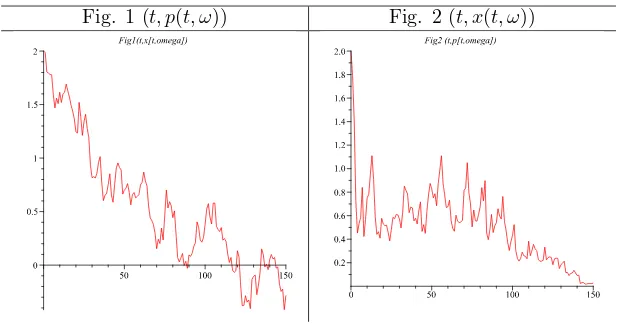
Example Let t ∈ Ω01 and the standard Wiener process W = (Wt)t∈Ω01. We
the cost functional. This problem means to find an optimal controlu∗ to bring the
Itˆo dynamical system from the originx0 at time t to a terminal point x1, which is unspecified, timet= 1 such as to maximize the objective functionalJ.
The control Hamiltonian 1−form is
H(t, xt, ut, pt, qt) =
the critical pointut=p2t, for the coefficient function ofdt, is a maximum point. On
the other hand, the adjoint systemdpt=−∂x∂Ht+ptdWtbecomesdpt=−dt+ptdWt.
Also, since the pointx1is unspecified, the transversality condition impliesp(1) = 0. It follows the costatept=e−
, the optimal controlu∗
t =
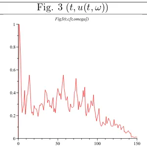
The numerical simulation can be done using the Euler method for the following equation of evolutiondx(t) = (p(t)/2)dt+dW(t) and the adjoint equation dp(t) = −dt+p(t)dW(t).We obtain the orbits: (t, p(t, ω)), (t, x(t, ω)), (t, u(t, ω)).
Fig. 3 (t, u(t, ω))
5
Optimal feedback control of a
continuously monitored spin
The dynamics of thecontinuously monitored spin systemis described by the SDEs [7]
drt=
1 2(
η rt−
rt) sin2θtdt+√η (1−r2t) cosθtdWt
dθt=
µ
−ut+ (
η r2
t
−η−12) sin2θtcosθt
dt+√η sinθt rt
dWt,
where thepolar coordinates(r, θ) represent the state space, the parameter η ∈[0,1] is thedetection efficiency of the photodetectors and ut is the amplitude of the
mag-netic field applied in they-direction. The special case η = 1 meansperfect detector efficiency.
Remark. Letting the initial value ofr equal to 1 (r0 = 1) we see thatdr0 = 0 and hence rt= 1, ∀t ≥0. Hence, r = 1 is a forward invariant setof the foregoing
stochastic dynamics. Physically, this means that if the detection is perfect, a pure state of the system will remain pure for all time.
We pose now the following optimization problem: Suppose that at time t the state of the system is (r, θ). Letus, s∈[0, T] (T is the time at which the experiment
terminates) be a square integrable function. We define the following expected cost-to-go
J(u(·)) =E
·Z
Ω0T
µ
−1 2u
2
t−U(rt, θt)
dt
¸
,
where the expectation value is taken with respect to every possible sample path that starts at (r, θ) at timet. The functionU is a measure of the distance of the state from the desired target state (r, θ) = (1,0). For well-posedness we require thatU(1,0) = 0 andU(r, θ)>0,∀(r, θ)6= (1,0). For example, U = 1−rcosθ. We seek the control lawuthat maximizesJ.
The control Hamiltonian 1−form is
H=
µ
−12u2t−U(rt, θt)
+p1
6
Ramsey and Uzawa-Lucas stochastic models
Ramsey stochastic modelsWe suppose that an investor is able to invest his wealth to do some products and he can get profit from this activity. Letx(t) be the capital of investor, a(t) the labor and c(t) > 0 the rate of consumption, at time t. Since there must be some risk in the investment, the Ramsey deterministic model [11]
dx(t) = (f(x(t), a(t))−c(t))dtcan be changed into a stochastic model
dx(t) = (f(x(t), a(t))−c(t))dt+σ(x(t))dW(t),
whereW(t) is a 1-dimensional standard Wiener process andσis aC1 function. For
simplicity, we introduce the following assumptions: (1) the functionf is given by the Cobb-Douglas formulaf(x, a) =kxαaβ, wherek, α, βare some constants; (2) during
a relatively short period we can takea(t) =a= constant.Ifβ= 1, then the stochastic evolution is
dx(t) = (kaxα(t)−c(t))dt+σ(x(t))dW(t), x(0) =x0.
We propose to maximize the performance function
J(c(·)) =E
In this case, the control Hamiltonian stochastic 1-form is
H(t, xt, ct, pt) =e−rt
cγ(t)
γ dt+pt(kax
α(t)
−c(t)−σ′(x(t))σ(x(t)))dt.
Applying the Theorem 4.1, it follows
fixes the optimal stochastic state evolution
dx(t) =³kaxα(t)−e−rt
γ−1 p(t) 1
γ−1 ´
dt+σ(x(t))dW(t) and the optimal stochastic costate evolution
dp(t) =−p(t)¡αkax(t)α−1−σ′′(x(t))σ(x(t))−σ′(x(t))2¢dt
−p(t)σ′(x(t))dW(t).
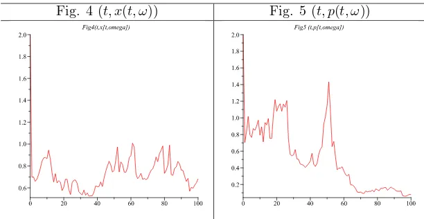
The simulations refer to
σ(x) =1 2x
2;k= 0.005;a= 1000;γ= 0.8;r= 0.3;α= 0.5.
The figures 4 and 5 represent the orbits: (t, x(t, ω)) and (t, p(t, ω)), respectively. Fig. 4 (t, x(t, ω)) Fig. 5 (t, p(t, ω))
Uzawa-Lucas stochastic models The Uzawa-Lucas deterministic model [5] (first published in 1965 by Uzawa [18] and reconsidered in 1988 by Lucas [9]), refers to a two sector economy: (1) a good sector that produces consumable and gross in-vestment in physical capital; (2) an education sector that produces human capital. Both are subject to maunder conditions of constant returns to scale. All the variables are also accepted asper capitaquantities. Let introduce the following data: kis the physical capital,his a human capital, c is the realper capitaconsumption, uis the fraction of labor allocated to the production of physical capital,β is the elasticity of output with respect to physical capital,ρ > 0 is a positive discount factor,γ >0 is the constant technological level in the good sector,δ >0 is the constant technological level in the education sector,nis the exogenous growth rate of labor,σ−1 is the con-stant of the elasticity of intertemporal substitution, andσ6=β. Given the importance of the sustainable development process, a modern economic approach regarding the role of human capital in economic growth in the case of the Romanian economy, using deterministic Uzawa-Lucas model, is done in [1].
The Uzawa-Lucas deterministic problem:
max
u,c J(u(·), c(·)) =
Z
Ω0T
e−ρt c(t)1−σ−1
subject to
dk(t) =¡γk(t)βu(t)1−β−nk(t)−c(t)¢dt, k(0) =k0, dh(t) =δ(1−u(t))h(t)dt, h(0) =h0
can be extended to the stochastic problem:
max
In this case, the control Hamiltonian stochastic 1-form is
H(t, xt, ct, pt, qt) =e−ρt
Applying the Theorem 4.1, it follows
dk(t) =¡γk(t)βu(t)1−βh(t)1−β−nk(t)−c(t)¢dt+σ1(k(t))dW(t) which fixes the optimal stochastic state evolution
and the optimal stochastic costate evolution
dp(t) =−p(t)¡γβ−k(t)1−βh(t)1−β−n−σ′′
1(k(t))σ1(k(t))−σ′1(k(t))2
¢
dt
−p(t)σ′
1(k(t))dW(t)
dq(t) =−q(t)¡¡δ(1−u(t))−σ2′′(h(t))σ2(h(t))−σ′2(h(t))2
¢
dt+σ′2(h(t))dW(t)
¢
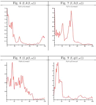
The simulations refer to
σ1(x) =σ2(x) =x;β= 0.25;γ= 1.05;
δ= 0.005;n= 0.01;ρ= 0.04;σ= 1.5, h0= 10;k0= 80.
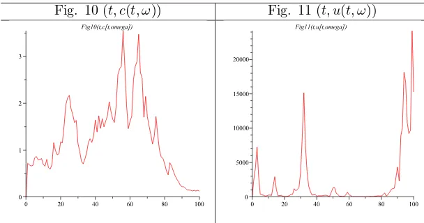
The figures 6, 7, 8, 9, 10 and 11 represent the orbits: (t, k(t, ω)), (t, h(t, ω)), (t, p(t, ω)), (t, q(t, ω)), (t, c(t, ω)), (t, u(t, ω)).
Fig. 6 (t, k(t, ω)) Fig. 7 (t, h(t, ω))
Fig. 10 (t, c(t, ω)) Fig. 11 (t, u(t, ω))
7
Conclusions
Alternatively to the classical stochastic control literature (e.g., [2], [10]), we start from a non-linear Itˆo differential system and we build a stochastic variational system and also an adjoint stochastic system. Both systems (variational and adjoint) are created considering a fixed control function. In order to prove the Theorem 4.1, regarding the single-time simplified stochastic maximum principle, we variate the control func-tion. Our approach is different from those existing in the classical literature. We also apply a geometrical formalism, using the integrand 1-form, in order to offer a way of changing the single-time problems into multitime problems (objective func-tionals given by curvilinear integrals or multiple integrals, constrained by multitime Itˆo evolution equations).
Acknowledgement Partially supported by Grant POS DRU/6/1.5/S/16, Uni-versity Politehnica of Bucharest. The authors would like to thank all those who have provided encouraging comments about the contents of this paper: Prof. Dr. Ionel T¸ evy (University Politehnica of Bucharest), Vasile Dr˘agan, Toader Morozan and Constantin Vˆarsan (Research Workgroup on Optimal Control from Institute of Mathematics of the Romanian Academy), Prof. Dr. Gheorghit¸˘a Zb˘aganu (University of Bucharest), Prof. Dr. Dumitru Opri¸s (West University of Timi¸soara) and Dr. Marius R˘adulescu (Institute of Mathematical Statistics and Applied Mathematics, Bucharest).
References
[1] M. Alt˘ar, C. Necula, G. Bobeic˘a,Modeling the economic growth in Romania. The role of human capital, Romanian Journal of Economic Forecasting, 9, 3 (2008), 115-128.
[2] A. Bensoussan, J. L. Lions, Impulse control and quasivariational inequalities, Gauthier-Villars, Montrouge, 1984.
[4] M. Bodnariu, Stochastic differential equalities and global limits, J. Adv. Math. Stud., 3, 2 (2010), 11-22.
[5] M. Ferrara, L. Guerrini,A note on the Uzawa-Lucas model with unskilled labor, Applied Sciences, 12 (2010), 90-95.
[6] A. Friedman,Stochastic Differential Equations and Applications, 2 Vol. Academic Press, 1976.
[7] S. Grivopoulos,Optimal Control of Quantum SystemsPhD Thesis, University of California, Santa Barbara, November 2005.
[8] N. El. Karoui, S. Peng, M.C. Quenez,Backward stochastic differential equations in finance, Math. Finance 7 (1997), 1-71.
[9] R. E. J. Lucas,On the mechanics of economic development, Journal of Monetary Economics, 22 (1988), 3-42.
[10] S. Peng, A general stochastic maximum principle for optimal control problems, SIAM J. Control and Optimization, 28, 4 (1990), 966-979.
[11] F. P. Ramsey, A mathematical theory of savings, The Economic Journal, 38 (1928), 543-559.
[12] C. Tudor, Stochastic Processes (Second edition) (in Spanish), Sociedad Matem´atica Mexicana, Guanajuato, Mexic, 1997.
[13] C. Udri¸ste,Lagrangians constructed from Hamiltonian systems, Mathematics and Computers in Business and Economics, WSEAS Press (2008), 30-33, MCBE-08, June 24-26, 2008, Bucharest, Romania.
[14] C. Udri¸ste,(2008).Multitime controllability, observability and Bang-Bang princi-ple, Journal of Optimization Theory and Applications, 139, 1 (2008), pp. 141-157. [15] C. Udri¸ste,Multitime stochastic control theory, Selected Topics on Circuits, Sys-tems, Electronics, Control & Signal Processing (eds. S. Kartalopoulos, M. Demi-ralp, N. Mastorakis, R. Soni, H. Nassar), WSEAS Press, (2007), 171-176. [16] C. Udri¸ste,Nonholonomic approach of multitime maximum principle, Balkan J.
Geom. Appl., 14, 2 (2009), 111-126.
[17] C. Udri¸ste,Simplified multitime maximum principle, Balkan J. Geom. Appl., 14, 1 (2009), 102-119.
[18] H. Uzawa,Optimum technical change in an aggregative model of economic growth, International Economic Review, 6 (1965), 18-31.
[19] C. Vˆarsan,On necessary conditions for stochastic control problems, Rev. Roum. Math. Pures et Appl., tome XXVIII, 7 (1983), pp. 641-663.
[20] J. Yong, X. Y. Zhou,Stochastic Controls: Hamiltonian Systems and HJB Equa-tions, Springer, New York, 1999.
Author’s address:
C. Udri¸ste, V. Damian,
UniversityPolitehnica of Bucharest, Faculty of Applied Sciences, Department of Mathematics-Informatics I, 313 Splaiul Independent¸ei, RO-060042 Bucharest, Romania.