El e c t ro n ic
Jo ur
n a l o
f P
r o
b a b il i t y
Vol. 16 (2011), Paper no. 26, pages 792–829. Journal URL
http://www.math.washington.edu/~ejpecp/
Quenched limits and fluctuations of the empirical measure
for plane rotators in random media
Eric Luçon
∗[email protected]
Abstract
The Kuramoto model has been introduced to describe synchronization phenomena observed in groups of cells, individuals, circuits, etc. The model consists ofN interacting oscillators on the one dimensional sphereS1, driven by independent Brownian Motions with constant drift chosen at random. This quenched disorder is chosen independently for each oscillator according to the same lawµ. The behaviour of the system for largeN can be understood via its empirical measure: we prove here the convergence asN → ∞of the quenched empirical measure to the unique solution of coupled McKean-Vlasov equations, under weak assumptions on the disorder µand general hypotheses on the interaction. The main purpose of this work is to address the issue of quenched fluctuations around this limit, motivated by the dynamical properties of the disordered system for large but fixed N: hence, the main result of this paper is a quenched Central Limit Theorem for the empirical measure. Whereas we observe a self-averaging for the law of large numbers, this no longer holds for the corresponding central limit theorem: the trajectories of the fluctuations process are sample-dependent.
Key words:Synchronization - quenched fluctuations - central limit theorem - disordered systems - Kuramoto model.
AMS 2000 Subject Classification:Primary 60F05, 60K37, 82C44, 92D25. Submitted to EJP on July 23, 2010, final version accepted March 17, 2011.
∗Laboratoire de Probabilités et Modèles Aléatoires (CNRS U.M.R. 7599) and Université Paris 6 – Pierre et Marie Curie,
1
Introduction
In this work, we study the fluctuations in the Kuramoto model, which is a particular case of interact-ing diffusions with a mean field Hamiltonian that depends on a random disorder. The Kuramoto model was first introduced in the 70’s by Yoshiki Kuramoto ([17], see also [1] and references therein) to describe the phenomenon of synchronization in biological or physical systems. More precisely, the Kuramoto model is a particular case of a system of N oscillators (considered as ele-ments of the one-dimensional sphereS1:=R/2πZ) solutions to the following SDE:
dxi,Nt = 1
N
N
X
j=1
b(xi,N,xj,N,ωj)dt+c(xi,N,ωi)dt+dBti, t∈[0,T], i=1 . . .N, (1)
where T >0 is a fixed (but arbitrary) time, bandc are smooth periodic functions. The Kuramoto case corresponds to a sine interaction (b(x,y,ω) =Ksin(y−x)andc(x,ω) =ω). This case which has the particularity of being rotationally invariant (namely, if(xi,N)i is a solution of the Kuramoto model,(xi,N+c)i,ca constant, is also a solution), will be referred to in this work as thesine-model. The parameter K > 0 is the coupling strength and (ωj) is a sequence of randomly chosen reals
(being i.i.d. realizations of a lawµ). The sequence(ωj)j is calleddisorderand represents the fact that the behaviour of each rotator xj,N depends on its own local frequencyωj.
Due to the mean field character of (1), the behaviour of the system can be understood via its empirical measureνN, process with values inM1(S1×R), that is the set of probability measures on oscillators and disorder:
∀(ω)∈RN, ∀t∈[0,T], νtN,(ω):=
1
N
N
X
j=1
δ(xj,N t ,ωj),
where(ω) = (ωj)j≥1is a fixed sequence of disorder inRN.
The purpose of this paper is to address the issue of both convergence and fluctuations of the empir-ical measure, asN → ∞; thus the main theorem of this paper (Theorem 2.10) concerns a Central Limit Theorem in a quenched set-up (namely the quenched fluctuations ofνN around its limit).
Some heuristic results have been obtained in the physical literature ([1] and references therein) concerning the convergence of the empirical measure, as N → ∞, to a time-dependent measure
(Pt(dx, dω))t∈[0,T], whose density w.r.t. Lebesgue measure at time t, qt(x,ω) is the solution of a deterministic non-linear McKean-Vlasov equation (see Eq.(5)). It is well understood ([1], [11]) that crucial features of this equation are captured in the sine-model by order parameters rt andψt
defined by:
rteiψt=
Z
S1×R
ei xqt(x,ω)dxµ(dω).
The quantity rt captures in fact the degree of synchronization of a solution (the profile qt ≡ 21π
for example corresponds to r =0 and represents a total lack of synchronization) andψt identifies
relation r= ΨK,µ(r), withΨK,µ(·)an explicit function such thatΨK,µ(0) =0. ForK small, r=0 is the only solution of such an equation and the system is not synchronized, but forKlarge, non-trivial solutions appear (synchronization). In the easiest instances, such a non-trivial solution is unique (in the sense thatr = ΨK,µ(r)admits a unique non-zero solution but of course one obtains an infinite number of solutions by rotation invariance that isψcan be chosen arbitrarily).
In[9], Dai Pra and den Hollander have rigorously shown the convergence of the averaged empirical measure LN ∈ M1(C([0,T],S1)× R) (probability measure on the whole trajectories and the disorder):
LN = 1
N
N
X
j=1
δ(xj,N,ω j).
This convergence of the law of LN under the joint law of the oscillators and the disorder is shown via an averaged large deviations principle in the case where b(x,y,ω) = K · f(y − x) and
c(x,ω) = g(x,ω) for f and g smooth and bounded functions. As a corollary, it is deduced in
[9]the convergence of LN and of νN, via a contraction principle, in the averaged set-up. In the case of unbounded disorder, the same proof can be generalized (thesis in preparation) under the following assumption:
∀t>0,
Z
R
et|ω|µ(dω)<∞. (HµA)
One aim of this paper is to obtain the limit of νN,(ω) in the quenched model, namely for a fixed
realization of the disorder(ω). This result can be deduced from the large deviations estimates in
[9], via a Borel-Cantelli argument, but our result is more direct and works under the much weaker assumption onµ,R
R|ω|µ(dω)<∞.
A crucial aspect of the quenched convergence result, which is a law of large numbers, is that it shows theself-averagingcharacter of this limit: every typical disorder configuration leads asN → ∞to the same evolution equation.
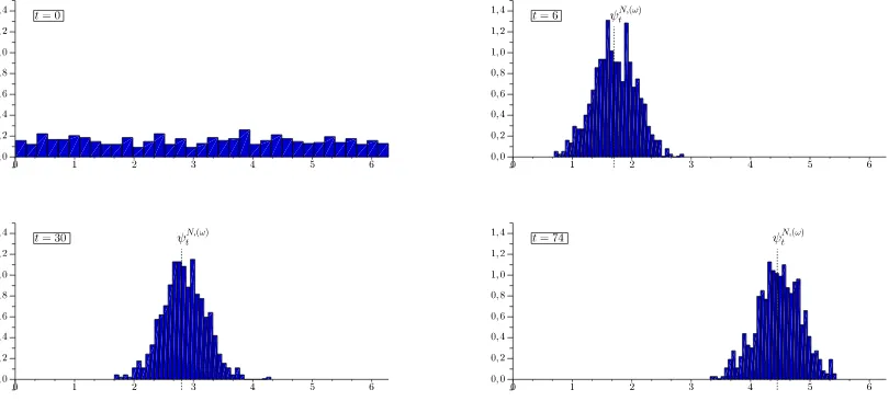
However, it seems quite clear even at a superficial level that if we consider the central limit theorem associated to this convergence, self-averaging does not hold since the fluctuations of the disorder compete with the dynamical fluctuations. This leads for example to a remarkable phenomenon (pointed out e.g. in[2]on the basis of numerical simulations): even if the distributionµ is sym-metric, the fluctuations of a fixed chosen sample of the disorder makes it not symmetric and thus the center of the synchronization of the systemslowly(i.e. with a speed of order 1/pN) rotates in one direction and with a speed that depends on the sample of the disorder (Fig. 1 and 2). This non-self averaging phenomenon can be tackled in the sine-model by computing the finite-size order parameters (Fig. 2):
rtN,(ω)eiψNt,(ω) = 1
N
N
X
j=1
ei xtj,N =
D
νtN,(ω),ei x
E
. (2)
Figure 1: We plot here the evolution of the marginal on S1 of νN,(ω) for N = 600 oscillators in the sine-model (µ= 1
2(δ−1+δ1), K = 6). The oscillators are initially chosen independently and
Figure 2: Trajectories of the center of synchronizationψN,(ω)in the sine-model for different realiza-tions of the disorder (µ= 12(δ−0.5+δ0.5),K=4,N=400). We observe here the non self-averaging
model of social interaction in an averaged set-up. Here we prove convergence in law of thequenched
fluctuations process
ηN,(ω):=pNνN,(ω)−P,
seen as a continuous process in the Schwartz spaceS′ of tempered distributions onS1×R to the solution of an Ornstein-Uhlenbeck process. The quenched convergence is here understood as a weak convergencein law w.r.t. the disorderand is more technically involved than the convergence in the averaged system. The main techniques we exploit have been introduced by Fernandez and Méléard
[12]and Hitsuda and Mitoma [15], who studied similar fluctuations in the case without disorder. In[7], A Large Deviation Principle is also proved. We refer to Section 4 for detailed definitions.
While numerical computations of the trajectories of the limit process of fluctuations clearly show a non self-averaging phenomenon, the dynamical properties of the fluctuations process that we find are not completely understood so far. Progress in this direction requires a good understanding of the spectral properties of the linearized operator of McKean-Vlasov equation around its non-trivial stationary solution; the stability of the non-synchronized solution q ≡ 21π has been treated by Strogatz and Mirollo in[24]. In the particular case without disorder, spectral properties of the evolution operator linearized around the non-trivial stationary solution are obtained in[3], but the case with a general distributionµneeds further investigations.
This work is organized as follows: Section 2 introduces the model and the main results. Section 3 focuses on the quenched convergence ofνN. In Section 4, the quenched Central Limit Theorem is
proved. The last section 5 applies the fluctuations result to the behaviour of the order parameters in the sine-model.
2
Notations and main results
2.1
Notations
• ifX is a metric space,BX will be its Borelσ-field,
• Cb(X)(resp. Cbp(X), p=1, . . . ,∞), the set of bounded continuous functions (resp. bounded continuous with bounded continuous derivatives up to orderp) onX, (Xwill be oftenS1×R),
• Cc(X) (resp. Ccp(X), p = 1, . . . ,∞), the set of continuous functions with compact support
(resp. continuous with compact support with continuous derivatives up to orderp) onX,
• D([0,T],X), the set of right-continuous with left limits functions with values onX, endowed with the Skorokhod topology,
• M1(Y), the set of probability measures onY (Y topological space, with a regularσ-fieldB),
• MF(Y), the set of finite measures onY,
• (M1(Y),v): M1(Y) endowed with the topology of vague convergence, namely the coarsest topology onM1(Y)such that the evaluationsν7→R fdν are continuous, where f are contin-uous with compact support.
We will useC as a constant which may change from a line to another.
2.2
The model
We consider the solutions of the following system of SDEs:
fori=1, . . . ,N, forT>0, for all t≤T,
xi,Nt =ξi+ 1
N
N
X
j=1
Z t
0
b(xsi,N,xsj,N,ωj)ds+
Z t
0
c(xsi,N,ωi)ds+Bit, (3)
where the initial conditionsξiare independent and identically distributed with lawλ, and indepen-dent of the Brownian motion(B) = (Bi)i≥1, and whereb(resp.c) is a smooth function, 2π-periodic w.r.t. the two first (resp. first) variables. The disorder(ω) = (ωi)i≥1is a realization of i.i.d. random
variables with lawµ.
Remark 2.1.
The assumption that the random variables(ωi)are independent will not always be necessary and
will be weakened when possible.
Instead of consideringxi,N as elements ofR, we will consider their projection onS1. For simplicity, we will keep the same notationxi,N for this projection1.
We introduce the empirical measureνN (on the trajectories and disorder):
Definition 2.2.
For all t ≤ T , for a fixed trajectory(x1, . . . ,xN)∈ C([0,T],(S1)N)and a fixed sequence of disorder
(ω), we define an element ofM1(S1×R)by:
νtN,(ω)= 1
N
N
X
i=1
δ(xi,N t ,ωi).
Finally, we introduce the fluctuations processηN,(ω)ofνN,(ω)around its limitP(see Th. 2.5):
Definition 2.3.
For all t≤T , for fixed(ω)∈RN, we define:
ηN,t (ω)=pNνtN,(ω)−Pt.
Throughout this article, we will denote asPthe law of the sequence of Brownian Motions and asP the law of the sequence of the disorder. The corresponding expectations will be denoted asEandE respectively.
2.3
Main results
2.3.1 Quenched convergence of the empirical measure
In[9], Dai Pra and den Hollander are interested in theaveragedmodel, i.e. in the convergence in law of the empirical measureunder the joint law of both oscillators and disorder. The model studied here, which is more interesting as far as the biological applications are concerned isquenched: for a fixed realization of the disorder (ω), do we have the convergence of the empirical measure? Moreover the convergence is shown under weaker assumptions on the moments of the disorder.
We consider here the general case where b(x,y,ω) is bounded, Lipschitz-continuous, and 2π -periodic w.r.t. the two first variables. cis assumed to be Lipschitz-continuous w.r.t. its first variable, but not necessarily bounded (see the sine-model, where c(x,ω) =ω). We also suppose that the function ω 7→ S(ω) := supx∈S1|c(x,ω)| is continuous (this is in particular true if c is uniformly
continuous w.r.t. to both variables (x,ω), and obvious in the sine-model whereS(ω) = |ω|). The Lipschitz bounds forbandc are supposed to be uniform inω.
The disorder(ω), is assumed to be a sequence of identically distributed random variables (but not necessarily independent), such that the law of each ωi is µ. We suppose that the sequence (ω)
satisfies the following property: forP-almost every sequence(ω),
1
N
N
X
i=1
sup
x∈S1|
c(x,ωi)| →N→∞ Z
sup
x∈S1|
c(x,ω)|µ(dω)<∞. (HQµ)
We make the following hypothesis on the initial empirical measure:
ν0N,(ω)N−→→∞ν0, in law, in(M1(S1×R),w). (H0)
Remark 2.4. 1. The required hypotheses about the disorder and the initial conditions are weaker than for the large deviation principle:
• the (identically distributed) variables(ωi)need not be independent: we simply need a
convergence (similar to a law of large numbers) only concerning the functionS,
• Condition (HµQ) is weaker than (HµA) on page 796; for the sine-model, (HµQ) reduces to
R
|ω|µ(dω)<∞,
• the initial values need not be independent, we only assume a convergence of the empir-ical measure.
2. The hypothesis (HQµ) is verified, for example, in the case of i.i.d. random variables, or in the case of an ergodic stationary Markov process.
3. Under (H0), the second marginal ofν0 isµ.
In Section 3, we show the following:
Theorem 2.5.
Under the hypothesis(H0)and (HQµ), for P-almost every sequence(ωi), the random variableνN,(ω)
following weak equation (for every f continuous bounded onS1×R, twice differentiable, with bounded derivatives):
Pt, f
=ν0, f
+1
2
Z t
0
dsPs, f′′
+
Z t
0
dsPs, f′(b[·,Ps] +c)
, (4)
where
b[x,m] =
Z
b(x,y,π)m(dy, dπ).
Moreover, with the same hypotheses, the law ofνN under the joint law of the oscillators and disorder
(averaged model) converges weakly to P as well.
Remark 2.6.
An easy calculation shows that P can be considered as a weak solution to the family of coupled McKean-Vlasov equations (see[9]):
1. Pcan be written asP(dx, dω) =µ(ω)Pω(dx),
2. if we defineqωt through Pt(dx, dω) = µ(ω)qωt (dx), qωt is the unique weak solution of the McKean-Vlasov equation:
d dtq
ω
t =L
ωqω
t , q
ω
0 =λ. (5)
where,Lωis the following differential operator:
Lωqωt =− ∂
∂x
Z
R
b(x,y,π)qπt(dy)µ(dπ) +c(x,ω)
qωt
+1
2 ∂2 ∂x2q
ω
t . (6)
We insist on the fact that Eq. (5) is indeed a (possibly) infinite system of coupled non-linear PDEs. To fix ideas, one may consider the simple case where µ= 1
2(δ−1+δ1). Then (5) reduces to two
equations (one for+1, the other for−1) which are coupled via the averaged measure 1
2(q
+1
t +q−
1 t ).
But for more general situations (µ=N(0, 1)say) this would consist of an infinite number of coupled equations.
Remark 2.7 (Generalization to the non compact case).
The assumption that the state variables are inS1, although motivated by the Kuramoto model, is not absolutely essential: Theorem 2.5 still holds in the non-compact case (e.g. whenS1 is replaced by
Rd), under the additional assumptions of boundedness of x 7→ |c(x,ω)|and the first finite moment of the initial condition:R|x|λ(dx)<∞.
2.3.2 Quenched fluctuations of the empirical measure
Theorem 2.5 says that forP-almost every realization(ω)of the disorder, we have the convergence ofνN,(ω)towards P, which is a law of large numbers. We are now interested in the corresponding Central Limit Theorem associated to this convergence, namely, for afixedrealization of the disorder
(ω), in the asymptotic behaviour, asN → ∞of the fluctuations fieldηN,(ω)taking values in the set of signed measures:
∀t∈[0,T], ηtN,(ω):=pN
νtN,(ω)−Pt
.
In the case with no disorder, such fluctuations have already been studied by numerous authors (eg. Sznitman[25], Fernandez-Méléard[12], Hitsuda-Mitoma[15]). More particularly, Fernandez and Méléard show the convergence of the fluctuations field in an appropriate Sobolev space to an Ornstein-Uhlenbeck process.
Here, we are interested in thequenchedfluctuations, in the sense that the fluctuations are studied for fixed realizations of the disorder. We will prove a weak convergence of the law of the process ηN,(ω),in law w.r.t. the disorder.
In addition to the hypothesis made in §2.3.1, we make the following assumptions about b and c
(whereDpis the set of all differential operators of the form∂uk∂πl withk+l≤p):
b∈ Cb∞(S1×R), c∈ C∞(S1×R),
∃α >0, sup
D∈D6 Z
R
supu∈S1|Dc(u,π)|2
1+|π|2α dπ <∞,
(Hb,c)
Furthermore, we make the following assumption about the law of the disorder (α is defined in (Hb,c)):
the(ωj)are i.i.d. and
Z
R
|ω|4αµ(dω)<∞. (HµF)
Remark 2.8.
The regularity hypothesis aboutbandccan be weakened (namelyb∈ Cbn(S 1
×R)andc∈ Cm(S1× R)for sufficiently largenandm) but we have keptm=n=∞for the sake of clarity.
Remark 2.9.
In the case of the sine-model, Hypothesis (Hb,c) is satisfied withα=2 for example.
In order to state the fluctuations theorem, we need some further notations: for alls≤T, letLs be the second order differential operator defined by
Ls(ϕ)(y,π):= 1
2ϕ
′′(y,π) +ϕ′(y,π)(b[y,P
s] +c(y,π)) +
Ps,ϕ′(·,·)b(·,y,π).
LetW the Gaussian process with covariance:
E(Wt(ϕ1)Ws(ϕ2)) =
Z s∧t
0
¬
Pu,ϕ′1ϕ2′
¶
For allϕ1,ϕ2bounded and continuous onS1×R, let
Γ1(ϕ1,ϕ2) =
Z
R
Covλ ϕ1(·,ω),ϕ2(·,ω)
µ(dω), (8)
=
Z
S1×R
ϕ1−
Z
S1
ϕ1(·,ω)dλ
ϕ2−
Z
S1
ϕ2(·,ω)dλ
λ(dx)µ(dω),
and
Γ2(ϕ1,ϕ2) =Covµ Z
S1
ϕ1dλ,
Z
S1
ϕ2dλ
, (9)
=
Z
R Z
S1
ϕ1dλ−
Z
S1×R
ϕ1dλdµ
Z
S1
ϕ2dλ−
Z
S1×R
ϕ2dλdµ
dµ.
For fixed (ω), we may consider HN(ω), the law of the process ηN,(ω); HN(ω) belongs to
M1(C([0,T],S′)), where S′ is the usual Schwartz space of tempered distributions on S1×R. We are here interested in the law of the random variable(ω)7→ HN(ω)which is hence an element ofM1(M1(C([0,T],S′))).
The main theorem (which is proved in Section 4) is the following:
Theorem 2.10 (Fluctuations in the quenched model).
Under(HFµ),(Hb,c), the sequence(ω)7→ HN(ω)converges in law to the random variableω7→ H(ω), where H(ω) is the law of the solution to the Ornstein-Uhlenbeck process ηω solution in S′ of the following equation:
ηωt =X(ω) +
Z t
0 Ls∗η
ω
s ds+Wt, (10)
where,Ls∗ is the formal adjoint operator ofLs and for all fixedω, X(ω) is a non-centered Gaussian
process with covarianceΓ1 and with mean value C(ω). As a random variable inω, ω7→C(ω)is a Gaussian process with covarianceΓ2. Moreover, W is independent on the initial value X .
Remark 2.11.
In the evolution (10), the linear operatorLs∗ is deterministic ; the only dependence in ω lies in
the initial conditionX(ω), through its non trivial meansC(ω). However, numerical simulations of trajectories ofηω(see Fig. 3) clearly show a non self-averaging phenomenon, analogous to the one observed in Fig 2: ηωt not only depends on ω through its initial condition X(ω), but also for all positive timet>0.
Understanding how the deterministic operatorLs∗ propagates the initial dependence in ωon the
whole trajectory is an intriguing question which requires further investigations (work in progress). In that sense, one would like to have a precise understanding of the spectral properties ofLs∗, which appears to be deeply linked to the differential operator in McKean-Vlasov equation (6) linearized around its non-trivial stationary solution.
Remark 2.12 (Generalization to the non-compact case).
whereS1is replaced byRd. To this purpose, one has to introduce an additional weight(1+|x|α)−1in the definition of the Sobolev norms in Section 4 and to suppose appropriate hypothesis concerning the first moments of the initial conditionλ(R|x|βλ(dx)<∞for a sufficiently largeβ).
2.3.3 Fluctuations of the order parameters in the Kuramoto model
For givenN≥1, t∈[0,T]and disorder(ω)∈RN, let rNt ,(ω)>0 andζtN,(ω)∈S1 such that
rtN,(ω)ζN,t (ω)=
1
N
N
X
j=1
ei xtj,N =
D
νtN,(ω),ei x
E
.
Proposition 2.13 (Convergence and fluctuations forrtN,(ω)).
We have the following:
1. Convergence of rtN,(ω): ForP-almost every realization of the disorder, rN,(ω)converges in law in
C([0,T],R), to r defined by
t∈[0,T]7→rt:=
Pt, cos(·)
2
+Pt, sin(·)
212.
2. If r0>0then
∀t∈[0,T], rt>0. (Hr)
3. Fluctuations of rtN,(ω)around its limit: Let
t7→ RtN,(ω):=pNrtN,(ω)−rt
be the fluctuations process. For fixed disorder (ω), let RN,(ω) ∈ M1(C([0,T],R))
be the law of RN,(ω). Then, under (Hr), the random variable (ω) 7→ RN,(ω) con-verges in law to the random variable ω 7→ Rω, where Rω is the law of Rω :=
1
r 〈P, cos(·)〉 ·
ηω, cos(·)+〈P, sin(·)〉 ·ηω, sin(·).
Remark 2.14.
In simpler terms, this double convergence in law corresponds for example to the convergence in law of the corresponding characteristic functions (since the tightness is a direct consequence of the tightness of the process η); i.e. for t1, . . . ,tp ∈ [0,T] (p ≥ 1) the characteristic function of
(RtN,(ω)
1 , . . . ,R
N,(ω)
tp ) for fixed (ω) converges in law, as a random variable in (ω), to the random
characteristic function of(Rtω
1, . . . ,R ω
tp).
Proposition 2.15 (Convergence and fluctuations forζN,(ω)).
We have the following:
1. Convergence of ζN,(ω): Under(Hr), for P-almost every realization of the disorder (ω), ζN,(ω)
converges in law toζ:t∈[0,T]7→ζt:= 〈 Pt,ei x〉
Figure 3: We plot here the evolution of the imaginary part of the processZω, for different realiza-tions ofω; the trajectories are sample-dependent, as in Fig 2.
2. Fluctuations ofζN,(ω)around its limit: Let
t7→ ZtN,(ω):=pNζN,t (ω)−ζt
be the fluctuations process. For fixed disorder(ω), letZN,(ω)∈ M1(C([0,T],R))be the law of
ZN,(ω). Then, under(Hr), the random variable (ω)7→ZN,(ω)converges in law to the random
variableω7→Zω, whereZωis the law ofZω:= r12
rηω, cos(·)+¬P,ei x¶Rω.
In the sine-model, we haveζN,(ω)=eiψN,(ω) whereψN,(ω)is defined in (2) and is plotted in Fig. 2. Some trajectories of the processZωare plotted in Fig. 3.
This fluctuations result is proved in Section 5.
3
Proof of the quenched convergence result
In this section we prove Theorem 2.5. Reformulating (3) in terms ofνN,(ω), we have:
∀i=1 . . .N, ∀t∈[0,T], xi,Nt =ξi+
Z t
0
b[xsi,N,νsN]ds+
Z t
0
c(xsi,N,ωi)ds+Bti, (11)
where we recall that b[x,m]:=R b(x,y,π)m(dy, dπ).
The idea of the proof of Theorem 2.5 is the following: we show the tightness of the sequence(νN,(ω))
separable and by an argument of boundedness of the second marginal of any accumulation point, thanks to (HµQ), we show the tightness inD([0,T],(MF,w)). The proof is complete when we prove the uniqueness of any accumulation point.
3.1
Proof of the tightness result
We want to show successively:
1. Tightness ofL(νN,(ω))inD([0,T],(MF,v)),
2. Equation verified by any accumulation point,
3. Characterization of the marginals of any limit,
4. Convergence inD([0,T],(MF,w)).
3.1.1 Equation verified byνN,(ω)
For f ∈ Cb2(S1×R), we denote by f′, f′′the first and second derivative off with respect to the first variable. Moreover, ifm∈ M1(S1×R), thenm, fstands forR
S1×Rf(x,π)m(dx, dπ).
Applying Ito’s formula to (11), we get, for all f ∈ Cb2(S1×R),
D
νtN,(ω), f
E
=
D
ν0N,(ω), f
E
+1
2
Z t
0
ds¬νsN,(ω), f′′¶
+
Z t
0
ds¬νsN,(ω), f′·(b[·,νsN,(ω)] +c)¶+MN,f(t),
whereMN,f(t):= N1
PN j=1
Rt 0 f
′(xN,(ω)
j ,ωj)dBj(s)is a martingale (f′bounded).
3.1.2 Tightness ofL(νN,(ω))in D([0,T],(MF,v))
Cc(S1×R)is separable: let(fk)k≥1(elements ofC∞(S1×R)) a dense sequence inCc(S1×R), and
let f0≡1. We defineΩ:=D([0,T],(M1,v))and the applicationsΠf, f ∈ Cc(S1×R)by:
Πf : Ω → D([0,T],R)
m 7→ m, f.
Let (Pn)n a sequence of probabilities on Ω and (ΠfPn) = Pn◦Π−f1 ∈D([0,T],R). We recall the following result:
Lemma 3.1.
If for all k≥0, the sequence(Πf
Hence, it suffices to have a criterion for tightness in D([0,T],R). Let Xnt be a sequence of processes in D([0,T],R) and Ftn a sequence of filtrations such that Xn is Fn-adapted. Let φn={stopping times forFn}. We have (cf. Billingsley[4]):
Lemma 3.2 (Aldous’ criterion).
If the following holds,
1. Lsupt≤TXn
, (Markov Inequality).
The tightness follows.
For allk≥1, we have the following decomposition:
At this point,L(νN,(ω))is tight inD([0,T],(MF,v)).
3.1.3 Equation satisfied by any accumulation point in D([0,T],(MF,v))
Using hypothesis (H0), it is easy to show that the following equation is satisfied for every
accumu-lation pointν, for everyf ∈ Cc2(S1×R)(we use here thatS1is compact):
νt, f=ν0, f
+
Z t
0
dsνs, f′·(b[·,νs] +c)+1
2
Z t
0
dsνs, f′′. (12)
For any accumulation pointν, the following lemma gives a uniform bound for the second marginal ofν:
Lemma 3.4.
Let Q be an accumulation point of L(νN,(ω))N in D([0,T],(M1,v)) and let beν ∼Q. For all t ∈
[0,T], we define by(νt,2)the second marginal ofνt:
∀A∈ B(R), (νt,2)(A) =
Z
S1×A
νt(dx, dπ).
Then, for all t∈[0,T],
Z
R sup
x∈S1|
c(x,π)|(νt,2)(dπ)≤
Z
R sup
x∈S1|
c(x,π)|µ(dπ).
Proof. Letφbe aC2positive function such thatφ≡1 on[−1, 1],φ≡0 on[−2, 2]andφ ∞≤1. Let,
∀k≥1, φk:=π7→φ
π
k
.
Thenφk ∈ Cc2(R) and φk(π) →k→∞ 1, for allπ. We have also for all π ∈R, |φk(π)| ≤
φ
∞,
|φk′(π)| ≤φ′
∞,|φ′′k(π)| ≤
φ′′
∞.
We have successively, denotingS(π):=supx∈S1|c(x,π)|, Z
S1×R
S(π)νt(dx, dπ) =
Z
S1×R
lim inf
k→∞ φk(π)S(π)νt(dx, dπ),
≤lim inf
k→∞
Z
S1×R
φk(π)S(π)νt(dx, dπ), (Fatou’s lemma),
=lim inf
k→∞ Nlim→∞
Z
S1×R
φk(π)S(π)ν N,(ω)
t (dx, dπ), (13)
≤ lim
N→∞
Z
S1×R
S(π)νtN,(ω)(dx, dπ), (since
φ
∞≤1).
The equality (13) is true since(x,π)7→φk(π)S(π)is of compact support inS1×R(recall thatS is
But, by definition ofνtN,(ω), and using the hypothesis (HQµ) concerningµ, we have,
lim
N→∞
Z
S1×R
S(π)νtN,(ω)(dx, dπ) =
Z
R
S(π)µ(dπ). (14)
The result follows.
Remark 3.5.
(14) is only true forP-almost every sequence(ω). We assume that the sequence(ω)given at the beginning satisfies this property.
3.1.4 Tightness in D([0,T],(MF,w))
We have the following lemma (cf. [21]):
Lemma 3.6.
Let (Xn) be a sequence of processes in D([0,T],(MF,w)) and X a process belonging to C([0,T],(MF,w)). Then,
Xn
L
→X⇔
(
Xn→L X inD([0,T],(MF,v)),
Xn, 1→ 〈L X, 1〉 inD([0,T],R).
So, it suffices to show, for any accumulation pointν:
1. 〈ν, 1〉 = 1: Eq. (12) is true for all f ∈ C2
c(S1×R), so in particular for fk(x,π):=φk(π).
Using the boundedness shown in lemma 3.4, we can apply dominated convergence theorem in Eq. (12). We then haveνt, 1
=1, for all t∈[0,T]. The fact that Eq. (12) is verified for all f ∈ C2
b(S
1×R)can be shown in the same way.
2. Continuity of the limit: For all 0≤s≤t≤T, for all f ∈ Cb2(S1×R),
νt, f−νs, f
≤K
Z t
s
νu, f′·b[·,νu]
du+1
2
Z t
s
νu, f′′du
+
Z t
s
νu, f′·cdu≤C× |t−s|, for some constantC.
Noticing that we used again Lemma 3.4 to bound the last term, we have the result.
Remark 3.7.
It is then easy to see that the second marginal (on the disorder) of any accumulation point isµ.
3.2
Uniqueness of the limit
Proposition 3.8.
There exists a unique element P ofD([0,T],MF(S1×R))which satisfies equation(12), P0∈ M1 and
P0,2=µ.
Remark 3.9.
Since this proof is an adaptation of Oelschläger[20]Lemma 10, p.474, we only sketch the proof:
We can rewrite Eq. (12) in a more compact way:
Pt, f=P0, f+
Z t
0
Ps, L(Ps)(f)ds, ∀f ∈ Cb2(S1×R), 0≤t≤T, (15)
where,
L(P)(f)(x,ω):= 1
2f
′′(x,ω) +h(x,ω,P)f′(x,ω), ∀x ∈S1,
∀ω∈R,
and,
h(x,π,P) =b[x,P] +c(x,π).
Lett7→Ptbe any solution of Eq. (15). One can then introduce the following SDE (whereξ∈Rand
˜
ξ∈S1 is its projection onS1):
¨
dξt = h(ξ˜t,ωt,Pt)dt+dWt, ξ0=ξ˜0, (ξ˜0,ω0)∼P0,
dωt = 0.
(16)
Eq. (16) has a unique (strong) solution(ξt,ωt)t∈[0,T]= (ξt,ω0)t∈[0,T]. The proof of uniqueness in Eq. (12) consists in two steps:
1. Pt=L(ξ˜t,ωt), for all t∈[0,T],
2. Uniqueness of ˜ξ.
We refer to Oelschläger[20]for the details. Another proof of uniqueness can be found in[9]or in
[13]via a martingale argument.
4
Proof of the fluctuations result
4.1
Distribution spaces
Let S := S(S1×R) be the usual Schwartz space of rapidly decreasing infinitely differentiable functions. LetDp be the set of all differential operators of the form∂uk∂πl withk+l ≤p. We know
from Gelfand and Vilenkin[14]p. 82-84, that we can introduce onS a nuclear Fréchet topology by the system of seminormsk · kp,p=1, 2, . . . , defined by
φ2
p=
p
X
k=0
Z
S1×R
(1+|π|2)2p X
D∈Dk
|Dφ(y,π)|2dydπ.
LetS′ be the corresponding dual space of tempered distributions. Although, for the sake of sim-plicity, we will mainly consider ηN,(ω) as a process in C([0,T],S′), we need some more precise estimations to prove tightness and convergence. We need here the following norms:
For every integer j, α∈R+, we consider the space of all real functions ϕ defined on S1×R with derivative up to order jsuch that
ϕ
j,α:=
X
k1+k2≤j Z
S1×R
|∂xk1∂πk2ϕ(x,π)|2
1+|π|2α dxdπ
1/2
<∞.
LetW0j,α be the completion ofCc∞(S1×R)for this norm;(W0j,α,k · kj,α)is a Hilbert space. LetW−
j,α
0
be its dual space.
LetCj,α be the space of functionsϕwith continuous partial derivatives up to order j such that
lim |π|→∞xsup∈S1
|∂xk1∂πk2ϕ(x,π)|
1+|π|α =0, for allk1+k2≤ j,
with norm
ϕ
Cj,α= X
k1+k2≤j
sup
x∈S1
sup
π∈R
|∂xk1∂πk2ϕ(x,π)|
1+|π|α .
We have the following embeddings:
W0m+j,α,→Cj,α,m>1,j≥0,α≥0,
i.e. there exists some constantC such that
ϕ
Cj,α≤C ϕ
m+j,α. (17)
Moreover,
W0m+j,α,→W0j,α+β,m>1,j≥0,α≥0,β >1.
Thus there exists some constantC such that
ϕ
j,α+β≤C ϕ
m+j,α.
We then have the following dual continuous embedding:
W0−j,α+β ,→W0−(m+j),α, m>1,α≥0,β >1. (18)
It is quite clear thatS ,→W0j,α for any jandα, with a continuous injection.
Lemma 4.1.
For every x,y∈S1,ω∈R, for allα, the linear mappings W03,α→Rdefined by
Dx,y,ω(ϕ):=ϕ(x,ω)−ϕ(y,ω);Dx,ω:=ϕ(x,ω);Hx,ω=ϕ′(x,ω),
are continuous and
Dx,y,ω
−3,α≤C|x−y|(1+|ω|
α), (19)
Dx,ω
−3,α≤C(1+|ω|
α), (20)
Hx,ω
−3,α≤C(1+|ω|
α). (21)
Proof. Letϕbe a function of classC∞with compact support onS1×R, then,
|ϕ(x,ω)−ϕ(y,ω)| ≤ |x− y|sup
u
ϕ′(u,ω),
≤ |x− y|(1+|ω|α)sup
u,ω
ϕ′(u,ω)
1+|ω|α !
,
≤ |x− y|(1+|ω|α)ϕ
1,α,
≤C|x−y|(1+|ω|α)ϕ
3,α,
following (17) with j =1 andm=2>1. Then, (19) follows from a density argument. (20) and (21) are proved in the same way.
4.2
The non-linear process
The proof of convergence is based on the existence of the non-linear process associated to McKean-Vlasov equation. Such existence has been studied by numerous authors (eg. Dawson[10], Jourdain-Méléard[16], Malrieu[18], Shiga-Tanaka[23], Sznitman[25],[26]) mostly in order to prove some propagation of chaos properties in systems without disorder. We consider the present similar case where disorder is present. Let us give some intuition of this process. One can replace the non-linearity in Eq. (5) by an arbitrary measurem(dx, dω):
∂tqωt = 1
2∂x xq
ω
t −∂x
(b[x,m] +c(x,ω))qωt .
In this particular case, it is usual to interpretqωt as the time marginals of the following diffusion:
d xωt =d Bt+b[xωt ,m]d t+c(x
ω
t ,ω)d t, ω∼µ.
It is then natural to consider the following problem, wheremis replaced by the proper measureP: on a filtered probability space(Ω,F,Ft,B,x0,Q), endowed with a Brownian motionB and with a
F0 measurable random variablex0, we introduce the following system:
xωt = x0+
Rt 0 b[x
ω
s ,Ps]ds+
Rt 0c(x
ω
s ,ω)ds+Bt,
ω ∼ µ,
Pt = L(xt,ω),∀t∈[0,T].
Proposition 4.2.
There is pathwise existence and uniqueness for Equation(22).
Proof. The proof is the same as given in Sznitman[26], Th 1.1, p.172, up to minor modifications. The main idea consists in using a Picard iteration in the space of probabilities onC([0,T],S1×R)
endowed with an appropriate Wasserstein metric. We refer to it for details.
4.3
Fluctuations in the quenched model
The key argument of the proof is to explicit the speed of convergence asN→ ∞for the rotators to the non-linear process (see Prop. 4.3).
A major difference between this work and [12] is that, since in our quenched model, we only integrate w.r.t. oscillatorsand notw.r.t. the disorder, one has to deal with remaining terms, seeZN
in Proposition 4.3, to compare with[12], Lemma 3.2, that would have disappeared in theaveraged model. The main technical difficulty of Proposition 4.3 is to control the asymptotic behaviour of such terms, see (24). As in[12], having proved Prop. 4.3, the key argument of the proof is a uniform estimation of the norm of the processηN,(ω), see Propositions 4.4 and 4.8, based on the generalized stochastic differential equation verified byηN(ω), see (30).
4.3.1 Preliminary results
We consider here a fixed realization of the disorder (ω) = (ω1,ω2, . . .). On a common filtered
probability space (Ω,F,Ft,(Bi)i≥1,Q), endowed with a sequence of i.i.d. Ft-adapted Brownian motions (Bi) and with a sequence of i.i.d. F0 measurable random variables(ξi) with law λ, we define asxi,N the solution of (11), and as xωi the solution of (22), with the same Brownian motion
Bi and with the same initial valueξi.
The main technical proposition, from which every norm estimation ofηN,(ω)follows is the following:
Proposition 4.3.
E
sup
t≤T
x
i,N
t −x
ωi t
2
≤C/N+ZN(ω1, . . . ,ωN), (23)
where the random variable(ω)7→ZN(ω)is such that:
lim
A→∞lim supN→∞ P
N ZN(ω)>A=0. (24)
The (rather technical) proof of Proposition 4.3 is postponed to the end of the document (see §A). Once again, we stress the fact that the termZN would have disappeared in the averaged model.
The first norm estimation of the process ηN,(ω)(which will be used to prove tightness) is a direct consequence of Proposition 4.3 and of a Hilbertian argument:
Proposition 4.4.
Under the hypothesis(HµF)onµ, the processηN,(ω)satisfies the following property: for all T >0,
sup
t≤T
E
ηN
,(ω)
t
2
−3,2α
where
Then, applying the latter equation to an orthonormal system (ϕp)p≥1 in the Hilbert spaceW3,2
α
0 ,
summing onp, we have by Parseval’s identity on the continuous functionalDxi,N
t ,x
On the other hand,
whereG(ϕ)(ω):=Rϕ(y,ωi)P
4.3.2 Tightness of the fluctuations process
Applying Ito’s formula to (11), we obtain, for allϕbounded function onS1×R, with two bounded derivatives w.r.t. x, for every sequence(ω), for all t≤T:
andMtN,(ω)(ϕ)is a real continuous martingale with quadratic variation process
And,
The result follows from the assumptions made onc.
Proposition 4.8.
Proof. Let(ψp)be a complete orthonormal system inW 6,α
0 ofC∞function onS1×Rwith compact
support. We prove the stronger result:
E
By Lemma 4.5, we have:
whereAN is defined in Proposition 4.4. The result follows.
Proposition 4.9. 1. For every N , for P-almost every(ω), the trajectories of the fluctuations process
ηN,(ω)are almost surely continuous in
S′,
2. For every N , forP-almost every(ω), the trajectories of MN,(ω)are almost surely continuous in
Proof. We only prove forMN,(ω), since, using Proposition 4.8, the proof is the same forηN,(ω). Let
(ϕp)be a complete orthonormal system inW−3,2
α
0 , then for every fixedN and(ω), we know from
the proof of Proposition 4.6, that for allǫ >0, there exists someM0>0 such that
X
p≥M0
sup
t≤T
(MtN,(ω)(ϕp))2<
ǫ 3,a.s.
Let(tm)be a sequence in[0,T]such thattm→m→∞ t.
M
N,(ω)
tm −M
N,(ω)
t
2
−3,2α= X
p≥1
MtN,(ω)
m −M
N,(ω)
t
2
(ϕp),
≤ M0 X
p=1
MtN,(ω)
m −M
N,(ω)
t
2
(ϕp) + 2ǫ
3 ≤ǫ,
if tmis sufficiently large.
We are now in position to prove the tightness of the fluctuations process. Let us recall some nota-tions: for fixed N and(ω)HN,(ω) is the law of the processηN,(ω). Hence,
HN,(ω) is an element ofM1(C([0,T],S′)), endowed with the topology of weak convergence and withB∗, the smallest σ-algebra such that the evaluationsQ7→Q, fare measurable, f being measurable and bounded. We will denote byΘN the law of the random variable(ω)7→ HN,(ω). The main result of this part is the following:
Theorem 4.10. 1. for P-almost every sequence (ω), the law of the process MN,(ω) is tight in
M1(C([0,T],S′)),
2. The law of the sequence(ω)7→ HN,(ω)is tight onM1 M1(C([0,T],S′)).
Before proving Theorem 4.10, we recall the following result and notations (cf. Mitoma[19], Th 3.1, p. 993):
Proposition 4.11 (Mitoma’s criterion).
Let(PN)be a sequence of probability measures on(CS′:=C([0,T],S′),BC
S ′). For eachϕ∈ S, we
denote byΠϕ the mapping ofCS′toC :=C([0,T],R)defined by
Πϕ:ψ(·)∈ CS′7→ψ(·),ϕ∈ C.
Then, if for allϕ∈ S, the sequence(PNΠ−ϕ1)is tight inC, the sequence(PN)is tight inCS′.
Remark 4.12.
A closer look to the proof of Mitoma shows that it suffices to verify the tightness of(PNΠ−ϕ1)forϕ in a countable dense subset of the nuclear Fréchet space(S,k · kp,p≥1).
• Condition[T]: for all t≤T andδ >0, there existsC>0 such that
This last term is lower or equal thanη1forδsufficiently small (depending on(ω)).
restriction, we can always suppose thatφj
6,α=1, for every j≥1. We define the following
decreasing sequences (indexed byJ≥1) of subsets ofM1 C([0,T],S′):
K1ǫ(ϕ1, . . . ,ϕJ):=
n
P;∀t,∀1≤ j≤J, PΠ−ϕ1
j satisfies(Tt,δ,C1) o
,
K2ǫ(ϕ1, . . . ,ϕJ):=
n
P;∀1≤ j≤J,∀η1,η2>0,PΠ−ϕ1j satisfies(Aη1,η2,C2) o
,
whereC1=C1(ǫ,δ),C2=C2(ǫ,η1,η2)will be precised later. By construction and by Mitoma’s
theorem (cf. Remark 4.12),
Kǫ:=\
J
(K1ǫ(ϕ1, . . . ,ϕJ)∩K2ǫ(ϕ1, . . . ,ϕJ))
is a relatively compact subset ofM1 C([0,T],S′). In order to prove tightness of(ΘN), it is sufficient to prove that, for allǫ >0,
∀i=1, 2, lim sup
N
ΘN [
J
Kiǫ(φ1, . . . ,φJ)c
!
≤ǫ. (33)
Forǫ >0, letA=A(ǫ)such that lim infN→∞P AN ≤A
≥1−ǫ, and
lim inf
N→∞ P
1
N
N
X
i=1
(1+|ωi|4α) +AN(ω1, . . . ,ωN)≤A
!
≥1−ǫ,
where AN is the random variable defined in Proposition 4.4. We define the corresponding
constants (for a sufficiently large constantC):
C1(ǫ,δ):=
r
A(ǫ)
δ , C2(ǫ,η1,η2):= η1η22
CA(ǫ).
Then,
ΘN(K1ǫ(φ1, . . . ,φJ))≥P
(ω), ∀t, ∀1≤ j≤J, ∀δ,
E
D
ηN,t (ω),φj
E
2
C1(δ,ǫ)2
≤δ
,
≥P
(ω), sup
t≤T
E
η
N,(ω)
t
2
−6,α
≤A
, (by definition ofC1),
≥P AN≤A(ǫ), (cf. (18) and (25)).
Letting J → ∞ in the latter inequality, we obtain: ΘN(SJK1ǫ(φ1, . . . ,φJ)c) ≤ P(AN > A).
Furthermore, forη2>0, 0< θ≤C2 andτN ≤T a stopping time, for all 1≤ j≤J,
4.3.3 Identification of the limit
The proof of the fluctuations result will be complete when we identify any possible limit.
Proposition 4.13 (Identification of the initial value).
The random variable(ω) 7→ Lη0N,(ω) converges in law to the random variable ω 7→ L(X(ω)), where for allω, X(ω) =C(ω) +Y , with Y a centered Gaussian process with covarianceΓ1. Moreover
ω7→C(ω)is a Gaussian process with covarianceΓ2, whereΓ1andΓ2are defined in(8)and(9).
Proof. For simplicity, we only identify here the law of
D
ηN,0 (ω),ϕEfor allϕ. The same proof works
for the law of finite-dimensional distributions
Γi forΓi(ϕ,ϕ),i=1, 2. One has:
D
η0N,(ω),ϕE=p1
N
N
X
i=1
ϕ(ξi,ωi)−
Z
S1
ϕ(x,ωi)λ(dx)
+p1
N
N
X
i=1
Z
S1
ϕ(x,ωi)λ(dx)−
ν0,ϕ
,
=:AN,(ω)+BN,(ω).
It is easy to see that BN,(ω) converges in law toZ2∼ N(0,Γ2). Moreover, forP-almost every(ω),
AN,(ω)converges in law toZ1∼ N(0,Γ1)(see Billingsley[5], Th. 27.3 p. 362). That means that for allu∈R,ψAN(u):=Eλ
eiuAN,(ω)
converges toψY(u):=e− u2
2Γ1. But, then, for all F∈ C
b(R),
E
F
Eλ
eiu
D
ηN0,(ω),ϕE
=EhFEλheiu(AN,(ω)+BN,(ω))ii=EhFeiuBN,(ω)ψN(u)
i
.
SinceψN(u)converges almost surely to a constant, the limit of the expression above exists (Slutsky’s
theorem) and is equal toE
F
eiuZ2−u 2 2Γ1
.
Proposition 4.14 (Identification of the martingale part).
ForP-almost every(ω), the sequence(MN,(ω))converges in law inC([0,T],S′)to a Gaussian process W with covariance defined in(7).
Proof. For fixed (ω), (MN,(ω)) is a sequence of uniformly square-integrable continuous martin-gales (cf. Remark 4.7), which is tight in C([0,T],S′). Let W1 and W2 be two accumulation points (continuous square-integrable martingales whicha priori depend on (ω)) and (Mφ(N),(ω))
and (Mψ(N),(ω)) be two subsequences converging to W1 and W2, respectively. Note that we can suppose that φ(N) ≤ ψ(N) for all N. For all ϕ ∈ S, limN→∞¬Mφ(N),(ω)(ϕ),Mψ(N),(ω)(ϕ)¶
t =
W1(ϕ),W2(ϕ)t, for all t, and
¬
Mφ(N),(ω)(ϕ),Mψ(N),(ω)(ϕ)¶t=
Z t
0
¬
νsφ(N),(ϕ′)2¶ds.
We now have to identify the limit: we already know that for P-almost every realization of the disorder(ω), (νN,(ω))converges in law to P. But, the latter expression, seen as a function ofν, is continuous. SoW1(ϕ),W2(ϕ)t =Rt
0
¬
Ps,(ϕ′)2¶. SoW1−W2 is a continuous square integrable martingale whose Doob-Meyer process is 0. SoW1=W2and is characterized as the Gaussian process
with covariance given in (7). The convergence follows.
Proof of the independence of W and X . We prove more : the triple(Y,C,W)is independent. For sake of simplicity, we only consider the case of(Y(ϕ),C(ϕ),Wt(ϕ))for fixedt andϕ.
Let us first recall some notations: letAN,(ω),BN,(ω)andMtN,(ω)(ϕ)be the random variables defined in the proof of Proposition 4.13 and 4.14 and letψAN(u):=E
eiuAN,(ω)
, ψBN(v) :=E
ei vBN,(ω)
,
ψMN(w):=E
eiw MtN,(ω)(ϕ)