Documenta Mathematica
Journal der
Deutschen Mathematiker-Vereinigung
Gegr¨
undet 1996
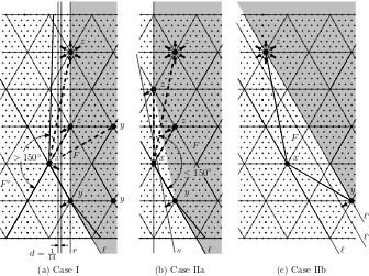
ℓ ℓ
r d= 1
14 ℓ
s
ℓ′′
>150◦ x x x
F′
F F
y ≤150◦
y F
z z
z z
z
z
y
ℓ′
(a) Case I (b) Case IIa (c) Case IIb y
y
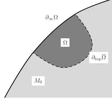
On Planar Graphs, cf. page 375
Documenta Mathematica, Journal der Deutschen Mathematiker-Vereinigung, ver¨offentlicht Forschungsarbeiten aus allen mathematischen Gebieten und wird in traditioneller Weise referiert. Es wird indiziert durch Mathematical Reviews, Science Citation Index Expanded, Zentralblatt f¨ur Mathematik.
Artikel k¨onnen als TEX-Dateien per E-Mail bei einem der Herausgeber eingereicht werden. Hinweise f¨ur die Vorbereitung der Artikel k¨onnen unter der unten angegebe-nen WWW-Adresse gefunden werden.
Documenta Mathematica, Journal der Deutschen Mathematiker-Vereinigung, publishes research manuscripts out of all mathematical fields and is refereed in the traditional manner. It is indexed in Mathematical Reviews, Science Citation Index Expanded, Zentralblatt f¨ur Mathematik.
Manuscripts should be submitted as TEX -files by e-mail to one of the editors. Hints for manuscript preparation can be found under the following WWW-address.
http://www.math.uni-bielefeld.de/documenta
Gesch¨aftsf¨uhrende Herausgeber / Managing Editors: Alfred K. Louis, Saarbr¨ucken [email protected]
Ulf Rehmann (techn.), Bielefeld [email protected] Peter Schneider, M¨unster [email protected]
Herausgeber / Editors:
Don Blasius, Los Angeles [email protected] Joachim Cuntz, M¨unster [email protected] Patrick Delorme, Marseille [email protected] Edward Frenkel, Berkeley [email protected] Kazuhiro Fujiwara, Nagoya [email protected] Friedrich G¨otze, Bielefeld [email protected] Ursula Hamenst¨adt, Bonn [email protected] Lars Hesselholt, Cambridge, MA (MIT) [email protected]
Max Karoubi, Paris [email protected]
Eckhard Meinrenken, Toronto [email protected] Alexander S. Merkurjev, Los Angeles [email protected] Anil Nerode, Ithaca [email protected]
Thomas Peternell, Bayreuth [email protected] Eric Todd Quinto, Medford [email protected]
Takeshi Saito, Tokyo [email protected] Stefan Schwede, Bonn [email protected] Heinz Siedentop, M¨unchen (LMU) [email protected]
Wolfgang Soergel, Freiburg [email protected] G¨unter M. Ziegler, Berlin (TU) [email protected]
ISSN 1431-0635 (Print), ISSN 1431-0643 (Internet)
SPARC
Leading Edge
Documenta Mathematica
Band 11, 2006
Igor Wigman
Statistics of Lattice Points
in Thin Annuli for Generic Lattices 1–23
Haruzo Hida
Automorphism Groups of Shimura Varieties 25–56
Sandra Rozensztajn
Compactification de Sch´emas Ab´eliens
D´eg´en´erant au-dessus d’un Diviseur R´egulier 57–71 W. Bley
On the
Equivariant Tamagawa Number Conjecture for Abelian Extensions
of a Quadratic Imaginary Field 73–118
Ernst-Ulrich Gekeler
The Distribution of Group Structures
on Elliptic Curves over Finite Prime Fields 119–142
Claude Cibils and Andrea Solotar Galois coverings, Morita Equivalence
and Smash Extensions of Categories over a Field 143–159 Bernd Ammann, Alexandru D. Ionescu, Victor Nistor
Sobolev Spaces on Lie Manifolds and
Regularity for Polyhedral Domains 161–206
Srikanth Iyengar, Henning Krause Acyclicity Versus Total Acyclicity
for Complexes over Noetherian Rings 207–240
Anton Deitmar and Joachim Hilgert
Erratum to: Cohomology of Arithmetic Groups with Infinite Dimensional Coefficient Spaces
cf. Documenta Math. 10, (2005) 199–216 241–241
Matthias Franz
Koszul Duality and Equivariant Cohomology 243–259
Christian B¨ohning
Derived Categories of Coherent Sheaves
on Rational Homogeneous Manifolds 261–331
Goro Shimura
Integer-Valued Quadratic Forms
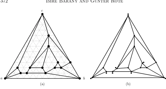
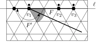
Imre B´ar´any and G¨unter Rote
Strictly Convex Drawings of Planar Graphs 369–391
Achill Sch¨urmann
On Packing Spheres into Containers 393–406
Philip Foth, Michael Otto A Symplectic Approach
to Van Den Ban’s Convexity Theorem 407–424
Henri Gillet and Daniel R. Grayson
Volumes of Symmetric Spaces via Lattice Points 425–447 Chia-Fu Yu
The Supersingular Loci and Mass
Formulas on Siegel Modular Varieties 449–468
Dabbek Khalifa et Elkhadhra Fredj
Documenta Math. 1
Statistics of Lattice Points
in Thin Annuli for Generic Lattices
Igor Wigman
Received: August 22, 2005
Communicated by Friedrich G¨otze
Abstract. We study the statistical properties of the counting func-tion of lattice points inside thin annuli. By a conjecture of Bleher and Lebowitz, if the width shrinks to zero, but the area converges to infinity, the distribution converges to the Gaussian distribution. If the width shrinks slowly to zero, the conjecture was proven by Hughes and Rudnick for the standard lattice, and in our previous paper for generic rectangular lattices. We prove this conjecture for arbitrary lattices satisfying some generic Diophantine properties, again assum-ing the width of the annuli shrinks slowly to zero. One of the obstacles of applying the technique of Hughes-Rudnick on this problem is the existence of so-called close pairs of lattice points. In order to overcome this difficulty, we bound the rate of occurence of this phenomenon by extending some of the work of Eskin-Margulis-Mozes on the quanti-tative Openheim conjecture.
2000 Mathematics Subject Classification: Primary: 11H06, Sec-ondary: 11J25
Keywords and Phrases: Lattice, Counting Function, Circle, Ellipse, Annulus, Two-Dimensional Torus, Gaussian Distribution, Diophan-tine approximation
1 Introduction
We consider a variant of the circle problem. Let Λ ⊂R2 be a planar lattice,
with det Λ the area of its fundamental cell. Let
2 Igor Wigman
denote its counting function, that is, we are counting Λ-points inside a disc of radiust.
As well known, as t → ∞, NΛ(t) ∼ det Λπ t2. Denoting the remainder or the
error term
∆Λ(t) =NΛ(t)− π
det Λt
2,
it is a conjecture of Hardy that
|∆Λ(t)| ≪ǫt1/2+ǫ.
Another problem one could study is thestatisticalbehavior of the value distri-bution of ∆Λ normalized by√t, namely of
FΛ(t) :=
∆Λ(t)
√ t .
Heath-Brown [HB] shows that for the standard lattice Λ =Z2, the value
dis-tribution ofFΛ, weakly converges to a non-Gaussian distribution with density p(x). Bleher [BL3] established an analogue of this theorem for a more general setting, where in particular it implies a non-Gaussian limiting distribution of
FΛ, for any lattice Λ⊂Z2.
However, the object of our interest is slightly different. Rather than counting lattice points in the circle of varying radiust, we will do the same forannuli. More precisely, we define
NΛ(t, ρ) :=NΛ(t+ρ)−NΛ(t),
that is, the number of Λ-points inside the annulus of inner radius tand width
ρ. The ”expected” value is the area π
det Λ(2tρ+ρ
2), and the corresponding
normalized remainder term is
SΛ(t, ρ) :=
NΛ(t+ρ)−NΛ(t)−det Λπ (2tρ+ρ2)
√
t .
The statistics of SΛ(t, ρ) vary depending to the size ofρ(t). Of our particular
interest is the intermediate or macroscopic regime. Here ρ → 0, but ρt → ∞. A particular case of the conjecture of Bleher and Lebowitz [BL4] states that SΛ(t, ρ) has a Gaussian distribution. In 2004 Hughes and Rudnick [HR]
established the Gaussian distribution for the unit circle, under an additional assumption that ρ(t)≫t−ǫ for everyǫ >0.
Statistics of Lattice Points . . . 3
Some of the work done in [W] extends quite naturally for the 2-parameter family of planar lattices 1, α+iβ. That is, in the current work we will require the algebraic independence ofαandβ, as well as a strong Diophantine property of the pair (α, β) (to be defined), rather than the transcendence and a strong Diophantine property of the aspect ratio of the ellipse, as in [W]. We say that a real numberξ isstrongly Diophantine, if for everyfixednatural
n, there existsK1>0, such that for integersaj with
It was shown by Mahler [MAH], that this property holds for a ”generic” real number. We say that a pair of numbers (α, β) is strongly Diophantine, if for everyfixednaturaln, there exists a numberK1>0, such that for every integral
polynomialp(x, y) = P
where the variance is given by
σ2:= 4π
β ·ρ. (2)
Remark: Note that the varianceσ2isα-independent, since the determinant
det(Λ) =β.
4 Igor Wigman
2 The distribution of S˜Λ, M, L
We apply the same smoothing as in [HR] and [W]: let χ be the indicator function of the unit disc and ψ a nonnegative, smooth, even function on the real line, of total mass unity, whose Fourier transform, ˆψ is smooth and has compact support. Introduce a rotationally symmetric function Ψ on R2 by
setting ˆΨ(~y) = ˆψ(|~y|), where | · | denotes the standard Euclidian norm. For
whereM =M(T) is the smoothing parameter, which tends to infinity with t. In this section, we are interested in the distribution of the smooth version of
SΛ(t, ρ), denoted ˜SΛ, M, L(t), whereL:= 1ρ, defined by assumption of theorem 1.1 regardingρ:= 1
L.
Rather than drawingtat random from [T,2T] with a uniform distribution, we prefer to work with smooth densities: introduce ω ≥0, a smooth function of total mass unity, such that bothω and ˆω are rapidly decaying, namely
|ω(t)| ≪ 1
(1 +|t|)A, |ωˆ(t)| ≪ 1 (1 +|t|)A, for every A >0. Define the averaging operator
hfiT =
and letPω, T be the associated probability measure:
Statistics of Lattice Points . . . 5
Remark: In what follows, we will suppress the explicit dependency on T, whenever convenient.
Theorem 2.1. Suppose that M(T) and L(T) are increasing to infinity with T, such that M = O(Tδ) for all δ > 0, and L/√M → 0. Then if (α, β)
is an algebraically independent strongly Diophantine pair, we have for Λ =
for any interval A, where
σ2:= 4π chine proved that almost alltuples inRn are Diophantine (see, e.g. [S], pages 60-63).
β. In the rest of the current section, we assume, that, unless specified otherwise, the set of the squared lengths of vectors in Λ∗satisfy the Diophantine property. That means, that (α2, αβ, β2) is a Diophantine
triple of real numbers. We may assume (α2, αβ, β2) being Diophantine, since
theorem 1.1 (and theorem 2.1) assume (α, β) isstrongly Diophantine, which is, obviously, a stronger assumption.
We use the following approximation to ˜NΛ,M(t) (see e.g [W], lemma 4.1), which holds unconditionally on any Diophantine assumption:
Lemma 2.2. As t→ ∞,
where, again, Λ∗ is the dual lattice.
6 Igor Wigman
One should note that ˆψbeing compactly supported means that the sum essen-tially truncates at|~k| ≈√M.
Unlike the standard lattice, clearly there are no nontrivial multiplicities in Λ, that is
Lemma2.4. Let a~j=mj+nj(α+iβ)∈Λ,j= 1,2, with an irrationalαsuch
that β /∈Q(α). Then if|a~1|=|a~2|, either n1=n2 andm1=m2 orn1=−n2 andn2=−m2.
Proof of theorem 2.1. We will show that the moments of ˜SΛ, M, L correspond-ing to the smooth probability space converge to the moments of the normal distribution with zero mean and variance which is given by theorem 2.1. This allows us to deduce that the distribution of ˜SΛ, M, L converges to the normal distribution asT → ∞, precisely in the sense of theorem 2.1.
First, we show that the mean isO(√1
due to the convergence of P ~ Then from (9), the binomial formula and the Cauchy-Schwartz inequality,
Statistics of Lattice Points . . . 7
Proposition 2.5 together with proposition 2.8 allow us to deduce the re-sult of theorem 2.1 for an algebraically independent strongly Diophantine (ξ, η) := (−α
β,
1
β). Clearly, (α, β) being algebraically independent and strongly Diophantine is sufficient.
2.1 The variance
The computation of the variance is done in two steps. First, we reduce the main contribution to the diagonal terms, using the assumption on the pair (α, β) (i.e. (α2, αβ, β2) is Diophantine). Then we compute the contribution of the diagonal terms. Both these steps are very close to the corresponding ones in [W].
Remark: In the formulation of proposition 2.5,K is implicitly given by (7).
Proof. Expanding out (10), we have
MΛ,2= 4
8 Igor Wigman
Recall that the support condition on ˆψmeans that~kand~lare both constrained to be of lengthO(√M). Thus the off-diagonal contribution (that is for|~k| 6=|~l|
Obviously, the contribution to (12) of the two last lines of (13) is negligible both in the diagonal and off-diagonal cases, justifying the diagonal approximation of (12) in the first statement of the proposition. To compute the asymptotics, we write we take a large parameter Y = Y(T)> 0 (to be chosen later), and
is a 2-dimensional Riemann sum of the integral
Statistics of Lattice Points . . . 9
2. We changed the coordinates
appropriately. And so,
This concludes the proposition, provided we have managed to choose Y with
L2 =o(Y) andY =o(M). Such a choice is possible by the assumption of the
proposition regardingL.
2.2 The higher moments
In order to compute the higher moments we will prove that the main contri-bution comes from the so-called diagonal terms (to be explained later). Our bound for the contribution of the off-diagonalterms holds for a strongly Dio-phantinepair of real numbers, which is defined below. In order to show that the strongly Diophantine pairs are ”generic”, we use theorem 2.6 below, which is a consequence of the work of Kleinbock and Margulis [KM]. The contribution of the diagonal terms is computed exactly in the same manner it was done in [W], and so we will omit it here.
Definition: We call the pair (ξ, η) strongly Diophantine, if for all natural
n there exists a number K1 = K1(ξ, η, n) ∈ N such that for every integral
Theorem2.6. Let an integernbe given. Then almost all pairs of real numbers
(ξ, η)∈R2 satisfy the following property: there exists a numberK
1=K1(n)∈ Nsuch that for every integer polynomial of2variablesp(x, y) = P
i+j≤n
ai, jxiyj
of degree≤n,(14)is satisfied.
10 Igor Wigman
Remark: Theorem A in [KM] is much more general than the result we are using. As a matter of fact, we have the inequality
The inequality above holds for every ǫ > 0 for a wide class of functions fi :
U →R, for almost allx∈U, whereU ⊂Rm is an open subset. Here we use this inequality for the monomials.
Remark: Simon Kristensen [KR] has recently shown, that the set of all pairs (ξ, η)∈R2 which fail to be strongly Diophantine has Hausdorff dimension 1.
Obviously, if (ξ, η) is strongly Diophantine, then any n-tuple of real numbers, which consists of a set of monomials in ξ and η, is Diophantine. Moreover, (ξ, η) is strongly Diophantine iff (−ξη, 1
η) is such.
We have the following analogue of lemma 4.7 in [W], which will eventually allow us to exploit the strong Diophantine assumption of (α, β).
Lemma 2.7. If (ξ, η) is strongly Diophantine, then it satisfies the following property: for any fixed naturalm, there existsK∈N, such that if
zj =a2j+b2jξ2+ 2ajbjξ+b2jη2≪M,
where the constant involved in the”≫” notation depends only onη andm.
The proof is essentially the same as the one of lemma 4.7 from [W], considering
the productQof numbers of the form Pm j=1
Statistics of Lattice Points . . . 11
Proof. Expanding out (10), we have
MΛ, m=
off-diagonal otherwise. Due to lemma 2.7, the contribution of theoff-diagonal
terms is:
for every A >0, by the rapid decay of ˆω and our assumption regardingM. Since m is constant, this allows us to reduce the sum to the diagonal terms. In order to be able to sum over all the diagonal terms we need the following analogue of a well-known theorem due to Besicovitch [BS] about incommensu-rability of square roots of integers.
Proposition2.9. Suppose thatξ andη are algebraically independent, and
zj=a2j+ 2ajbjξ+b2j(ξ2+η), (17)
such that(aj, bj)∈Z2+ are all different primitive vectors, for1≤j≤m. Then
{√zj}mj=1 are linearly independent overQ.
12 Igor Wigman
Definition: We say that a term corresponding to {k~1, . . . , ~km} ∈
Λ∗ \
{0}
m
and {ǫj} ∈ {±1}m is a principal diagonal term if there is a partition
{1, . . . , m}= l
F
i=1
Si, such that for each 1≤i≤l there exists a primitiven~i∈ Λ∗\ {0}, with non-negative coordinates, that satisfies the following property:
for every j ∈ Si, there exist fj ∈ Z with |k~j| = fj|n~i|. Moreover, for each 1≤i≤l, P
j∈Si
ǫjfj = 0.
Obviously, the principal diagonal is contained within the diagonal. However, the meaning of proposition 2.9 is, that in our situation, the converse also is true:
Corollary 2.10. Every diagonal term is a principle diagonal term whenether ξ andη are algebraically independent.
Computing the contribution of the principal diagonal terms is done literally the same way it was done in [W], and we sketch it here. As in [W], one can show
that the contribution of a particular partition{1, . . . , m}= l
F
i=1
Si is negligible, unlessm= 2l is even and #Si= 2 for all 1≤i≤l.
In the latter case, the contribution is asymptotic to 1. Therefore, the m -th moment is asymptotic to 0, if m is odd, and to the number of partitions {1, . . . , m} =
l
F
i=1
Si with #Si = 2 for all i, m = 2l. This number equals to m!
2m/2 m 2
!, which is also them-th moment of the standard Gaussian distribution.
3 Bounding the number of close pairs of lattice points
Roughly speaking, we say that a pair of lattice points, n and n′ is close, if
|n| − |n′|issmall. We would like to show that this phenomenon israre. This
is closely related to the Oppenheim conjecture, as |n|2
− |n′|2 is a quadratic
form on the coefficients of nandn′.
In order to establish a quantative result, we use a technique developed in a pa-per by Eskin, Margulis and Mozes [EMM]. Note that the proof is unconditional on any Diophantine assumptions.
3.1 Statement of the results
The ultimate goal of this section is to establish the following
Proposition3.1. LetΛ be a lattice and denote
Statistics of Lattice Points . . . 13
Then if δ >1, such that δ=o(R), we have
#A(R, δ)≪Rδ·logR
In order to prove this result, we note that evaluating the size of A(R, δ) is equivalent to counting integer points~v∈R4withT
≤ k~vk ≤2T such that
0≤Q1(v)≤δ,
whereQ1 is a quadratic form of signature (2,2), given explicitly by
Q1(~v) = (v1+v2α)2+ (v2β)2−(v3+v4α)2−(v4β)2. (19)
For a fixed δ >0 and a largeR, this situation was considered extensively by Eskin, Margulis and Mozes [EMM]. The authors give an asymptotical upper bound in this situation. We will examine how the constants involved in their bound depend on δ, and find out that there is a linear dependency, which is what we essentially need. The author wishes to thank Alex Eskin for his assistance with this matter.
Remarks: 1. In a more recent paper, Eskin Margulis and Mozes [EMM1] prove that for ”generic” lattice Λ, there is a constantc >0, such that for any
fixedδ >0, asR→ ∞, #A(R, δ) is asymptotic tocδR. 2. For our purposes we need a weaker result:
#A(R, δ)≪ǫRδ·Rǫ,
for everyǫ >0. If Λ is a rectangular lattice (i.e. α= 0), then this result follows from properties of the divisor function (see e.g. [BL], lemma 3.2).
Theorem 2.3 in [EMM] considers a more general setting than proposition 3.1. We state here theorem 2.3 from [EMM] (see theorem 3.2). It follows from theorem 3.3 from [EMM], which will be stated as well (see theorem 3.3). Then we give an outline of the proof of theorem 2.3 of [EMM], and inspect the dependency onδ of the constants involved.
3.2 Theorems 2.3 and 3.3 from [EMM]
Let ∆ be a lattice in Rn. We say that a subspace L
⊂ Rn is ∆-rational, if
L∩∆ is a lattice inL. We need the following definitions:
Definitions:
αi(∆) := sup
1
d∆(L)
Lis a ∆−rational subspace of dimensioni
,
where
14 Igor Wigman
Also
α(∆) := max
0≤i≤nαi(∆).
Since the space of unimodular lattices is canonically isomorphic to
SL(n,R)/SL(n, Z), the notation α(g) makes sense forg∈G:=SL(n,R). For a bounded functionf :Rn →R, with|f| ≤M, which vanishes outside a ballB(0, R), define ˜f :SL(n,R)→Rby the following formula:
˜
f(g) := X v∈Zn
f(gv).
Lemma 3.1 in [S2] implies that
˜
f(g)< cα(g), (20)
wherec=c(f) is an explicit constant constant
c(f) =c0Mmax(1, Rn),
for some constant c0 = c0(n), independent on f. In section 3.4 we prove a
stronger result, assuming some additional information about the support off. LetQ0be a quadratic form defined by
Q0(~v) = 2v1vn+ p
X
i=2 v2i −
nX−1
i=p+1 v2i.
Since
v1vn=
(v1+vn)2−(v1−vn)2
2 ,
Q0is of signaturep, q. Obviously,G:=SL(n,R) acts on the space of quadratic
forms of signature (p, q), and discriminant±1,O=O(p, q) by:
Qg(v) :=Q(gv).
Moreover, by the well known classification of quadratic forms, O is the orbit ofQ0 under this action.
In our case the signature is (p, q) = (2,2) andn= 4. We fix an elementh1∈G
withQh1=Q
1, whereQ1is given by (19). There exists a constantτ >0, such
that for everyv∈R4,
τ−1kvk ≤ kh1vk ≤τkvk. (21)
We may assume, with no loss of generality that τ≥1.
LetH :=StabQ0(G). Then the natural mophismH\G→ O(p, q) is a homeo-morphism. Define a 1-parameter familyat∈Gby:
atei=
e−te
1, i= 1
ei, i= 2, . . . , n−1
ete
n, i=n
Statistics of Lattice Points . . . 15
Clearly, at ∈H. Furthermore, let ˆK be the subgroup of G consisting of or-thogonal matrices, and denoteK:=H∩Kˆ.
Let (a, b) ∈ R2 be given and let Q : Rn
→ R be any quadratic form. The object of our interest is:
V(a, b)(Z) =V(Qa, b)(Z) ={x∈Z
n : a < Q(x)< b }.
Theorem 2.3 states, in our case:
Theorem 3.2 (Theorem 2.3 from [EMM]). Let Ω = {v ∈ R4| kvk <
The proof of theorem 3.2 relies on theorem 3.3 from [EMM], and we give here a particular case of this theorem
Theorem3.3(Theorem 3.3 from [EMM]). For any (fixed) lattice∆inR4,
sup
where the upper bound is universal.
3.3 Outline of the proof of theorem 3.2: Step 1: Define
Lemma 3.6 in [EMM] states that Jf is approximable by means of an integral over the compact subgroup K. More precisely, there is some constant C >0, such that for every ǫ >0,
Step 2: Choose a continuous nonnegative function f on R4
+ = {x1 > 0}
which vanishes outside a compact set so that
Jf(r, ζ)≥1 +ǫ
on [τ−1, 2τ]
16 Igor Wigman
Step 3: DenoteT =et, and suppose thatT
≤ kvk ≤2T anda≤Q0(h1v)≤ b. Then by (21),Jf kh1vkT−1, Q0(h1v)
≥1 +ǫ, and by (23), for a sufficiently larget,
C·T2 Z
K
f(atkh1v)dm(k)≥1, (24)
forT ≤ kvk ≤2T and
a≤Qx0(v)≤b. (25)
Step 4: Summing (24) over all v ∈ Z4 with (25) and T
≤ kvk ≤ 2T, we obtain:
#V(a, b)(Z)∩[T,2T]S3≤ X
v∈Zn C·T2
Z
K
f(atkh1v)dm(k)
=C·T2 Z
K ˜
f(atkh1)dm(k)
(26)
using the nonnegativity off.
Step 5: By (20), (26) is
≤C·c(f)·T2 Z
K
α(atkh1)dm(k).
Step 6: The result of theorem 2.3 is obtained by using theorem 3.3 on the last expression.
3.4 δ-dependency:
In this section we assume that (a, b) = (0, δ), which suits the definition of the set A(R, δ), (18). One should notice that there only 3δ-dependent steps: • Choosing f in step 2, such that Jf ≥ 1 +ǫ on [τ−1,2τ]×[0, δ]. We will construct a family of functionsfδ with an universal bound|fδ| ≤M, such that
fδ vanishes outside of a compact set which is only slightly larger than
V(δ) = [τ−1,2τ]×[−1, −1]2×[0, δτ
2 ]. (27)
This is done in section 3.4.1.
• The dependency ofT0 of step 3, so that the usage of lemma 3.6 in [EMM] is
legitimate. For this purpose we will have to examine the proof of this lemma. This is done in section 3.4.2.
• The constant c in (20). We would like to establish a linear dependency on
Statistics of Lattice Points . . . 17
3.4.1 Choosing fδ:
Notation: For a setU ⊂Rn, andǫ >0, denote
Uǫ:={x∈Rn: max
1≤i≤n|xi−yi| ≤ǫ,for somey∈U}.
Choose a nonnegative continuous function f0, onR4+, which vanishes outside
a compact set, such that its support,Ef0, slightly exceeds the set V(1). More precisely,V(1)⊂Ef0 ⊂V(1)δ0 for someδ0>0. By the uniform continuity of f, there are ǫ0, δ0 >0, such that if max
1≤i≤4|xi−x 0
i| ≤ δ0, then f(x)> ǫ0, for
every x0= (x0
1,0,0, x04)∈V(1).
Thus for (r, ζ) ∈ [τ−1,2τ]
×[0, δ], the contribution of [−δ0, δ0]2 to Jf0 is ≥ǫ0·(2δ0)2. Multiplyingf0 by a suitable factor, and by the linearity ofJf0, we may assume that this contribution is at least 1 +ǫ.
Now definefδ(x1, . . . , x4) :=f0(x1, x2, x3, xδ4). We have forδ≥1 ζ−x2
2+x23
2rδ = ζ/2r
δ −
(x2/
√ δ)2
2r +
(x3/
√ δ)2
2r .
Thus for δ ≥ 1, if (r, ζ) ∈ [τ−1,2τ]
×[0, δ] and for i = 2,3, |xi| < δ0, fδ satisfies:
fδ(r, x2, x3, x4)> ǫ0,
and therefore the contribution of this domain toJfδ is
≥ǫ0(2δ)2≥1 +ǫ
by our assumption.
By the construction, the family{fδ} has a universal upper boundM which is the one off0.
3.4.2 How large is T0
The proof of lemma 3.6 from [EMM] works well along the same lines, as long as
f(atx)6= 0 (28)
implies that for t → ∞, x/kxk converges to e1 = (1, 0,0,0). Now, since at preservesx1x4, (28) implies for the particular choice off =fδ in section 3.4.1:
|x1x4|=O(δ); x1≫T.
Thus
kxk=x1+O
δ T
+O(1),
18 Igor Wigman
3.4.3 Bounding integral points in Vδ: Lemma 3.4. Let V(δ)defined by
V(δ) = [τ−1,2τ]×[−1,−1]n−2×[0, δβ
2 ]. (29)
for some constant τ andn≥3. Letg∈SL(n,R)and denote N(g, δ) := #V(δ)∩gZn.
Then for δ≥1,
N(g, δ)−2
n−2(2τ−τ−1)δ
detg ≤c5δ
nX−1
i=1
1
vol(Li/(gZn∩Li)
for someg-rational subspacesLiofR4of dimensioni, wherec5=c5(n)depends only onn.
A direct consequence of lemma 3.4 is the following
Corollary 3.5. Let f : Rn
→ R be a nonnegative function which vanishes outside a compact set E. Suppose that E ⊂Vǫ(δ) for some ǫ > 0. Then for δ≥1,(20)is satisfied with
c(f) =c3·M δ, where the constant c3 depends onn only.
In order to prove lemma 3.4, we shall need the following:
Lemma 3.6. Let Λ⊂Rn be am-dimensional lattice, and let
At=
1 1
. .. t
(30)
an n-dimensional linear transformation. Then fort >0we have
detAtΛ≤tdet Λ. (31)
Proof. We may assume that m < n, since if m = n, we obviously have an equality. Let v1, . . . , vm the basis of Λ and denote for everyi,ui ∈Rn−1 the vector, which consists of first n−1 coordinates ofvi. Also, let xi ∈Rbe the last coordinate ofvi. By switching vectors, if necessary, we may assumex16= 0.
We consider the function
Statistics of Lattice Points . . . 19
x1 times the first row from any other, we obtain:
f(t) =
and by the multilinearity property of the determinant,f is a linear function of
t2. Write
≤0, being minus the determinant of a Gram matrix. Therefore,
(detAtΛ)2−t2det Λ =a(t2−1)≤0 fort≥1, implying (30).
Proof of lemma 3.4. We will prove the lemma, assuming β = 2. However, it implies the result of the lemma for anyβ, affecting onlyc5. Letδ >0. Trivially,
N(g, δ) =N(g0,1),
where g0 = A−δ1g with Aδ given by (30). Let λ1 ≤ λ2 ≤ . . . ≤ λn be the successive minima ofg0, and pick linearly independent lattice pointsv1, . . . , vn with kvik = λi. Denote Mi the linear space spanned by v1, . . . , vi and the
20 Igor Wigman
Thus, by the induction hypothesis, the number of such points is:
≤c4
4.1 An asymptotic formula for NΛ
We need an asymptotic formula for the sharp counting function NΛ. Unlike
the case of the standard lattice, Z2, in order to have a good control over the
error terms we should use some Diophantine properties of the lattice we are working with. We adapt the following notations:
Let Λ =h1, α+iβi, be a lattice, d:= det Λ =β its determinant, andt >0 a real variable. Denote the set of squared norms of Λ by
SNΛ={|~n|2: n∈Λ}.
Λ with consecutive increasing norms, choose~k:=n~1). We have the following
Statistics of Lattice Points . . . 21
Sketch of proof. The proof of this lemma is essentially the same as the one of lemma 5.1 in [W]. We start from
ZΛ(s) := 1
where the series is convergent forℜs >1.
The function ZΛ has an analytic continuation to the whole complex plane,
except for a single pole ats= 1, defined by the formula
Γ(s)π−sZΛ(s) =
Moreover,ZΛ satisfies the following functional equation:
ZΛ(s) =1
dχ(s)ZΛ∗(1−s), (32)
with
χ(s) =π2s−1Γ(1−s)
Γ(s) . (33)
The connection betweenNΛ andZΛ is given in the following formula, which is
satisfied for everyc >1:
22 Igor Wigman
The result of the current lemma follows from moving the contour of the inte-gration to the left, collecting the residue ats= 1 (see [W] for details).
Proposition 4.2. Let a lattice Λ =h1, α+iβi with a Diophantine triple of numbers(α2, αβ, β2)be given. Suppose thatL→ ∞asT → ∞and chooseM, such that L/√M →0, butM =O Tδ for every δ >0 as T → ∞. Suppose
furthermore, that M =O(Ls0)for some (fixed) s
0>0. Then *
SΛ(t, ρ)−S˜Λ, M, L(t)
2+
≪ √1 M
The proof of proposition 4.2 proceeds along the same lines as the one of propo-sition 5.1 in [W], using again an asymptotic formula for the sharp counting function, given by lemma 4.1. The only difference is that here we use proposi-tion 3.1 rather than lemma 5.2 from [W].
Once we have proposition 4.2 in our hands, the proof of our main result, namely, theorem 1.1 proceeds along the same lines as the one of theorem 1.1 in [W].
Acknowledgement. This work was supported in part by the EC TMR networkMathematical Aspects of Quantum Chaos, EC-contract no HPRN-CT-2000-00103 and the Israel Science Foundation founded by the Israel Academy of Sciences and Humanities. This work was carried out as part of the author’s PHD thesis at Tel Aviv University, under the supervision of prof. Ze´ev Rudnick. The author wishes to thank Alex Eskin for his help as well as the anonymous referees. A substantial part of this work was done during the author’s visit to the university of Bristol.
References
[BL] Pavel M. Bleher and Joel L. Lebowitz Variance of Number of Lattice Points in Random Narrow Elliptic Strip Ann. Inst. Henri Poincare, Vol 31, n. 1, 1995, pages 27-58.
[BL2] Pavel M. BleherDistribution of the Error Term in the Weyl Asymptotics for the Laplace Operator on a Two-Dimensional Torus and Related Lattice ProblemsDuke Mathematical Journal, Vol. 70, No. 3, 1993
[BL3] Bleher, Pavel On the distribution of the number of lattice points inside a family of convex ovalsDuke Math. J. 67 (1992), no. 3, pages 461-481.
[BL4] Bleher, Pavel M. ; Lebowitz, Joel L. Energy-level statistics of model quantum systems: universality and scaling in a lattice-point problem J. Statist. Phys. 74 (1994), no. 1-2, pages 167-217.
Statistics of Lattice Points . . . 23
[EMM] Eskin, Alex; Margulis, Gregory; Mozes, Shahar Upper bounds and asymptotics in a quantitative version of the Oppenheim conjecture Ann. of Math. (2) 147 (1998), no. 1, pages 93-141.
[EMM1] Eskin, Alex; Margulis, Gregory; Mozes, Shahar Quadratic forms of signature (2,2) and eigenvalue spaces on rectangular 2-tori, Ann. of Math. 161 (2005), no. 4, pages 679-721
[HB] Heath-Brown, D. R. The distribution and moments of the error term in the Dirichlet divisor problemActa Arith. 60 (1992), no. 4, pages 389-415.
[HR] C. P. Hughes and Z. Rudnick On the Distribution of Lattice Points in Thin Annuli International Mathematics Research Notices, no. 13, 2004, pages 637-658.
[KM] Kleinbock, D. Y., Margulis, G. A. Flows on homogeneous spaces and Diophantine approximation on manifolds Ann. of Math. (2) 148 (1998), no. 1, pages 339-360.
[KR] S. Kristensen,Strongly Diophantine pairs, private communication.
[MAH] K. Mahler Uber das Mass der Menge aller S-Zahlen¨ Math. Ann. 106 (1932), pages 131-139.
[S] Wolfgang M. SchmidtDiophantine approximationLecture Notes in Math-ematics, vol. 785. Springer, Berlin, 1980.
[S2] Schmidt, Wolfgang M. Asymptotic formulae for point lattices of bounded determinant and subspaces of bounded heightDuke Math. J. 35 1968 327-339.
[W] I. WigmanThe distribution of lattice points in elliptic annuli, to be pub-lished in Quarterly Journal of Mathematics, Oxford, available online in http://qjmath.oxfordjournals.org/cgi/content/abstract/hai017v1
Igor Wigman
School of Mathematical Sciences Tel Aviv University
Tel Aviv 69978 Israel
Documenta Math. 25
Automorphism Groups of Shimura Varieties
Haruzo Hida
Received: April 14, 2003 Revised: February 5, 2006
Communicated by Don Blasius
Abstract. In this paper, we determine the scheme automorphism group of the reduction modulopof the integral model of the connected Shimura variety (of prime-to-plevel) for reductive groups of typeA
andC. The result is very close to the characteristic 0 version studied by Shimura, Deligne and Milne-Shih.
2000 Mathematics Subject Classification: 11G15, 11G18, 11G25 Keywords and Phrases: Shimura variety, reciprocity law
There are two aspects of the Artin reciprocity law. One is representation theoretic, for example,
Homcont(Gal(Qab/Q),C×)∼= Homcont((A(∞))×/Q× +,C×)
via the identity ofL–functions. Another geometric one is:
Gal(Qab/Q)∼=GL
1(A(∞))/Q×+.
They are equivalent by duality, and the first is generalized by Langlands in non-abelian setting. Geometric reciprocity in non-abelian setting would be via Tannakian duality; so, it involves Shimura varieties.
Iwasawa theory is built upon the geometric reciprocity law. The cyclo-tomic field Q(µp∞) is the maximal p–ramified extension of Q fixed by
b Z(p)
⊂ A×/Q×R×
+ removing the p–inertia toric factor Z×p. We then try to study arithmetically constructed modules X out of Q(µp∞)⊂Qab. The main idea is to regard X as a module over over the Iwasawa algebra (which is a completed Hecke algebra relative to GL1(A(∞))
GL1(bZ(p))Q×+
26 Haruzo Hida
If one wants to get something similar in a non-abelian situation, we really need a scheme whose automorphism group has an identification withG(A(∞))/Z(Q)
for a reductive algebraic groupG. IfG=GL(2)/Q, the towerV/Qab of modular curves has Aut(V/Q) identified withGL2(A(∞))/Z(Q) as Shimura proved. The
decomposition group of (p) is given byB(Qp)×SL2(A(p∞))/{±1} for a Borel
subgroup B, and I have been studying various arithmetically constructed modules over the Hecke algebra of GL2(A(∞))
GL2(bZ(p))U(Zp)Q×+
, relative to the unipotent
subgroup U(Zp)⊂ B(Zp) (removing the toric factor from the decomposition group). Such study has yielded a p–adic deformation theory of automorphic forms (see [PAF] Chapter 1 and 8), and it would be therefore important to study the decomposition group at p of a given Shimura variety, which is basically the automorphism group of the modpShimura variety.
Iwasawa theoretic applications (if any) are the author’s motivation for the investigation done in this paper. However the study of the automorphism group of a given Shimura variety has its own intrinsic importance. As is clear from the construction of Shimura varieties done by Shimura ([Sh]) and Deligne ([D1] 2.4-7), their description of the automorphism group (of Shimura varieties of characteristic 0) is deeply related to the geometric reciprocity laws generalizing classical ones coming from class field theory and is almost equivalent to the existence of the canonical models defined over a canonical algebraic number field. Except for the modulopmodular curves and Shimura curves studied by Y. Ihara, the author is not aware of a single determination of the automorphism group of the integral model of a Shimura variety and of its reduction modulo p, although Shimura indicated and emphasized at the end of his introduction of the part I of [Sh] a good possibility of having a canonical system of automorphic varieties over finite fields described by the adelic groups such as the ones studied in this paper.
We shall determine the automorphism group of mod p Shimura varieties of PEL type coming from symplectic and unitary groups.
1 Statement of the theorem
LetB be a central simple algebra over a fieldM with a positive involutionρ
(thus TrB/Q(xxρ)>0 for all 06=x∈B). LetF be the subfield ofM fixed by
ρ. ThusF is a totally real field, and either M =F or M is a CM quadratic extension ofF. We writeO (resp. R) for the integer ring ofF (resp. M). We fix an algebraic closure F of the prime fieldFp of characteristicp > 0. Fix a proper subset Σ of rational places including ∞ and p. Let F+× be the subset
of totally positive elements inF, andO(Σ)denotes the localization of O at Σ
(disregarding the infinite place in Σ) andOΣis the completion ofOat Σ (again
Automorphism Groups of Shimura Varieties 27
exact sequence
1→B×/M×→Autalg(B)→Out(B)→1,
and by a theorem of Skolem-Noether, Out(B)⊂Aut(M). Here b∈ B× acts
on B by x 7→ bxb−1. Since B is central simple, any simple B-module N is
isomorphic each other. Take one such simple B-module. Then EndB(N) is a division algebraD◦. Taking a base of N overD◦ and identifyingN ∼= (D◦)r, we have B = EndD◦(N)∼=Mr(D) for the opposite algebraD ofD◦. Letting Autalg(D) act onb∈Mr(D) entry-by-entry, we have Autalg(D)⊂Autalg(B), and Out(D) = Out(B) under this isomorphism.
Let OB be a maximal order ofB. Let L be a projective OB–module with a non-degenerateF-linear alternating formh, i:LQ×LQ→F forLA=L⊗ZA
such that hbx, yi = hx, bρy
i for all b ∈ B. Identifying LQ with a product
of copies of the column vector space Dr on which Mr(D) acts via matrix multiplication, we can let σ ∈ Autalg(D) act component-wise on LQ so that
σ(bv) =σ(b)σ(v) for allσ∈Autalg(D).
LetC be the opposite algebra ofC◦= EndB(LQ). ThenC is a central simple
algebra and is isomorphic toMs(D), and hence Out(C)∼= Out(D) = Out(B). We write CA = C ⊗Q A, BA = B⊗QA and FA = F ⊗QA. The algebra
C has involution ∗ given by hcx, yi= hx, c∗yi for c ∈ C, and this involution “∗” ofC extends to an involution again denoted by “∗” of EndQ(LQ) given by
TrF/Q(hgx, yi) = TrF/Q(hx, g∗yi) forg∈EndQ(LQ). The involution∗(resp. ρ)
induces the involution∗ ⊗1 (resp. ρ⊗1) onCA (resp. onBA) which we write as ∗(resp. ρ) simply. Define an algebraic groupG/Q by
G(A) =g∈CA
ν(g) :=gg∗∈(FA)× forQ-algebrasA (1.1)
and an extension Ge of G by the following subgroup of the opposite group Aut◦A(LA) of theA-linear automorphism group AutA(LA):
e
G(A) =g∈Aut◦A(LA)
gCAg−1=CA and ν(g) :=gg∗∈(FA)× . (1.2)
Since C◦ = EndB(L
Q), we have B◦ = EndC(LQ), and from this we
find that gBg−1 = B
⇔ gCg−1 = C for g
∈ AutQ(LQ), and if this
holds for g, then gg∗ ∈ F× ⇔ gxρg−1 = (gxg−1)ρ for all x
∈ B and
gy∗g−1 = (gyg−1)∗ for all y ∈ C. Then G is a normal subgroup of Ge
of finite index, and Ge(Q)/G(Q) = OutQ-alg(C,∗). Here OutQ-alg(C,∗) is
the outer automorphism group of C commuting with ∗; in other words, it is the quotient of the group of automorphisms of C commuting with ∗ by the group of inner automorphisms commuting with ∗. Thus we have OutQ-alg(C,∗) ⊂ H0(h∗i,OutQ-alg(C)) ⊂ OutQ-alg(C) ⊂ Aut(M/Q). All the
28 Haruzo Hida
put P G=G/Z andPGe=G/Ze for the centerZ ofG.
We writeG1 for the derived group ofG; thus, G1 ={g ∈G|NC(g) =ν(g) =
1} for the reduced norm NC of C over M. We write ZG = G/G1 for the
cocenter of G. Then g 7→ (ν(g), NC(g)) identifies ZG with a sub-torus of ResF/QGm×ResM/QGm. IfM =F,G1 is equal to the kernel of the similitude
mapg7→ν(g); so, in this case, we ignore the right factor ResM/QGmand regard
ZG ⊂ResF/
QGm. By a result of Weil ([W]) combined with an observation in
[Sh] II (4.2.1), the automorphism group AutA-alg(CA,∗) of the algebra CA preserving the involution ∗ is given by PGe(A). In other words, we have an exact sequence of Q-algebraic groups
1→P G(A)→AutA-alg(CA,∗)(=PGe(A))→OutA-alg(BA, ρ)→1. (1.3) We write
π:Ge(A)→Ge(A)/G(A) = OutA-alg(BA, ρ)⊂OutA-alg(BA)
for the projection.
The automorphism group of the Shimura variety of level away from Σ is a quotient of the following locally compact subgroup ofGe(A(Σ)):
G(Σ)=nx
∈Ge(A(Σ))π(x)
∈OutQ-alg(B, ρ) o
, (1.4)
where we embed OutQ-alg(B, ρ) into Qℓ6∈ΣOutQℓ-alg(Bℓ) = OutA(Σ)-alg(B⊗Q
A(Σ)) by the diagonal map (B
ℓ=B⊗QQℓ).
We suppose to have an R–algebra homomorphism h : C → CR such that
h(z) =h(z)∗ and
(h1) (x, y) =hx, h(i)yiinduces a positive definite hermitian form onLR.
We define X to be the conjugacy classes of hunderG(R). ThenX is a finite disjoint union of copies of the hermitian symmetric domain isomorphic to
G(R)+/Ch, where C
h is the stabilizer of hand the superscript “+” indicates the identity connected component of the Lie groupG(R). Then the pair (G, X) satisfies the three axioms (see [D1] 2.1.1.1-3) specifying the data for defining the Shimura variety Sh(and its field of definition, the reflex fieldE; see [Ko] Lemma 4.1). In [D1], two more axioms are stated to simplify the situation: (2.1.1.4-5). These two extra axioms may not hold generally for our choice of (G, X) (see [M] Remark 2.2).
The complex points ofShare given by
Sh(C) =G(Q)\G(A(∞))
Automorphism Groups of Shimura Varieties 29
This variety can be characterized as a moduli variety of abelian varieties up to isogeny with multiplication byB. For eachx∈X, we havehx:C→CRgiven
by z 7→ g·h(z)g−1 for g
∈ G(R)/Ch sending hto x. Then v 7→ hx(z)v for
z∈Cgives rise to a complex vector space structure onLR, andXx(C) =LR/L
is an abelian variety, because by (h1),h, iinduces a Riemann form onL. The multiplication byb∈OB is given by (v modL)7→(b·v modL).
We suppose
(h2) all rational primes in Σ are unramified inM/Q, and Σ contains ∞and
p;
(h3) For every primeℓ∈Σ,OB,ℓ=OB⊗ZZℓ∼=Mn(Rℓ) forRℓ=R⊗ZZℓ;
(h4) For every primeℓ∈Σ,h, iinducesLℓ=L⊗ZZℓ∼= Hom(Lℓ, Oℓ); (h5) The derived subgroup G1 is simply connected; so, G1(R) is of type A
(unitary groups) or of typeC (symplectic groups).
LetG(ZΣ) ={g∈G(QΣ)|g·LΣ=LΣ} forQΣ=Q⊗ZZΣandLΣ=L⊗ZZΣ.
We define Sh(Σ) = Sh/G(ZΣ). This moduli interpretation (combined with
(h1-4)) allows us to have a well definedp–integral model of level away from Σ (see below for a brief description of the moduli problem, and a more complete description can be found in [PAF] 7.1.3). In other words,
Sh(Σ)(C) =G(Q)\G(A(∞))
×X/Z(Q)G(ZΣ)
has a well defined smooth model over OE,(p) :=OE⊗ZZ(p) which is again a
moduli scheme of abelian varieties up to prime-to–Σ isogenies. We writeSh(p)
forSh(Σ)when Σ ={p,∞}. We also writeQ(p)
Σ =QΣ/Qp andZ (p)
Σ =ZΣ/Zp.
We have taken full polarization classes under scalar multiplication by O×(Σ)+
in our moduli problem (while Kottwitz’s choice in [Ko] is a partial class of multiplication by Z×(Σ)+). By our choice, the group G is the full similitude
group, while Kottwitz choice is a partial rational similitude group. Our choice is convenient for our purpose because G has cohomologically trivial center, and the special fiber at p of the characteristic 0 Shimura variety Sh/G(ZΣ) gives rise to the modpmoduli of abelian varieties of the specific type we study (as shown in [PAF] Theorem 7.5), while Kottwitz’s modpmoduli is a disjoint union of the reduction modulo p of finitely many characteristic 0 Shimura varieties associated to finitely many different pairs (Gi, Xi) with Gi locally isomorphic each other at every place ([Ko] Section 8).
We fix a strict henselization W ⊂ Q of Z(p). Thus W is an unramified
30 Haruzo Hida
modular varieties and that of [Ra] for Hilbert modular varieties, Fujiwara ([F] Theorem in§0.4) proved the existence of a smooth toroidal compactification of
Sh(Sp)=Sh(p)/S for sufficiently small principal congruence subgroups S with
respect toLinG(A(p)) as an algebraic space over a suitable open subscheme of Spec(OE) containing Spec(W ∩E). Although our moduli problem is slightly different from the one Kottwitz considered in [Ko], as was done in [PAF] 7.1.3, following [Ko] closely, the p-integral moduli Sh(p) over O
E,(p) is proven to
be a quasi-projective scheme; so, Fujiwara’s algebraic space is a projective scheme (if we choose the toroidal compactification data well). If the reader is not familiar with Fujiwara’s work, the reader can take the existence of the smooth toroidal compactification (which is generally believed to be true) as an assumption of our main result.
Sincepis unramified inM/Q,OE,(p)is contained inW. We fix a geometrically
connected component V/Q of Sh(Σ)×
E Q and write V/W for the schematic
closure of V/Q in Sh(Σ)/W := Sh(Σ)/O
E,(p) ⊗OE,(p) W. By Zariski’s connectedness theorem combined with the existence of a normal projective compactification (either minimal or smooth) of Sh(Σ)/W, the reduction V/F = V ×WF is a
geo-metrically irreducible component of Sh(Σ)/W⊗WF. The schemeSh(Σ)/S classifies, for any S–scheme T, quadruples (A, λ, i, φ(Σ))/T defined as follows: A is an
abelian scheme of dimension 12rankZL for which we define the Tate module
T(A) = lim
←−NA[N], T
(Σ)(A) =
T(A)⊗ZZb(Σ), TΣ(A) = T(A)⊗Z ZΣ and
V(Σ)(A) = T(A)⊗
Z A(Σ); The symbol i stands for an algebra embedding
i : OB ֒→ End(A) taking the identity to the identity map on A; φ(Σ) is a level structure away from Σ, that is, anOB–linearφ(p):L⊗QA(p)∼=V(p)(A)
moduloG(ZΣ), where we require thatφ(Σp):L⊗ZQΣ(p) ∼=TΣ(A)⊗ZQ(Σp) send
L⊗ZZ(Σp) isomorphically ontoTΣ(A)⊗ZZ(Σp);λis a class of polarizationsλup
to scalar multiplication byi(O(Σ)+× ) which induces the Riemann form h·,·i on
Lup to scalar multiplication byO×(Σ)+. There is one more condition (cf. [Ko] Section 5 or [PAF] 7.1.1 (det)) specifying the module structure of ΩA/T over
OB⊗ZOT (which we do not recall).
The group G(A(Σ)) acts on Sh(Σ) by φ(Σ)
7→ φ(Σ)
◦ g. We can extend the action of G(A(Σ)) to the extension
G(Σ). Each element g
∈ G(Σ)
with projection π(g) = σg in OutQ-alg(B, ρ) acts also on Sh(Σ) by
(A, λ, i, φ(Σ))/T 7→(A, λ, i◦σ
g, φ(Σ)◦g)/T.
Automorphism Groups of Shimura Varieties 31
NC : Ge →ResM/QGm independently of the choice of A). The diagonal map
µ : Ge ∋ g 7→ (ν(g), NC(g)) ∈ (ResF/QGm×ResM/QGm) factors through the
cocenter ZG of G; so, we have a homomorphism µ : Ge
→ ZG of algebraic
Q-groups. We writeZG(R)+ for the identity connected component ofZG(R) and put ZG(Z(Σ))+ = ZG(R)+
∩O(Σ)× ×R×(Σ); so, ZG(Z(Σ))+ = O× (Σ)+ if M =F. Similarly, we identifyZ with ResR/ZGmso thatZ(Z(Σ)) =R×(Σ). We now state the main result:
Theorem 1.1. Suppose (h1-5). Then the field automorphism group
Aut(F(V)/F) of the function field F(V) over F is given by the stabilizer the connected componentV (inπ0(Sh(Σ)/F )) insideG(Σ)/Z(Z(Σ)). The stabilizer
is given by
GV =
n
g∈ G(Σ)µ(g)
∈ZG(Z(Σ))+o
Z(Z(Σ)) ,
whereZG(Z(Σ))+(resp. Z(Z(Σ))) is the topological closure ofZG(Z(Σ))+ (resp. Z(Z(Σ)))in ZG(A(Σ)) (resp. in G(A(Σ))). In particular, this implies that the scheme automorphism group Aut(V/F) coincides with the field automorphism
groupAut(F(V)/F)and is given as above.
This type of theorems in characteristic 0 situation has been proven mainly by Shimura, Deligne and Milne-Shih (see [Sh] II, [D1] 2.4-7 and [MS] 4.13), whose proof uses the topological fundamental group ofV and the existence of the analytic universal covering space. Our proof uses the algebraic fundamen-tal group of V and the solution of the Tate conjecture on endomorphisms of abelian varieties over function fields of characteristicpdue to Zarhin (see [Z], [DAV] Theorem V.4.7 and [RPT]). The characteristic 0 version of the finiteness theorem due to Faltings (see [RPT]) yields a proof in characteristic 0, arguing slightly more, but we have assumed for simplicity that the characteristic of the base field is positive (see [PAF] for the argument in characteristic 0). We shall give the proof in the following section and prove some group theoretic facts necessary in the proof in the section following the proof. Our original proof was longer and was based on a density result of Chai (which has been proven under some restrictive conditions on G), and Ching-Li Chai suggested us a shorter proof via the results of Zarhin and Faltings (which also eliminated the extra assumptions we imposed). The author is grateful for his comments.
2 Proof of the theorem
We start with
32 Haruzo Hida
isomorphism U ∼=σ(U). For x∈(U∩σ(U))(F), the two abelian varieties Xx
andXσ(x)are isogenous overF, whereXxis the abelian variety sitting overx.
Proof. We recall the subgroup in the theorem:
GV =
n
g∈ G(Σ)µ(g)∈ZG(Z(Σ))+o
Z(Z(Σ)) .
By characteristic 0 theory in [D] Theorem 2.4 or [MS] p.929 (or [PAF] 7.2.3), the action of Ge(A(Σ))/Z(Z(Σ)) on π
0(Sh(Σ)/Q) factors through the
homomor-phism Ge(A(Σ))/Z(Z(Σ))
→ ZG(A(Σ))/ZG(Z(Σ))+ induced by µ. The idele
class group of cocenter ZG(A(Σ))/ZG(Z(Σ))+ acts onπ
0(Sh(Σ)/Q) faithfully.
Since each geometrically connected component ofSh(Σ)is defined over the field
K of fractions of W, by the existence of a normal projective compactification (either smooth toroidal or minimal) over W (and Zariski’s connectedness theorem), we have a bijection between geometrically connected components overK and over the residue fieldFinduced by reduction modulo p. Then the stabilizer inGe(A(Σ))/Z(Z(Σ)) ofV in π
0(Sh(Σ)/F ) is given byGV.
The scheme theoretic automorphism group Aut(V /F) is a subgroup of the field automorphism group Aut(F(V)/F). By a generalization due to N. Jacobson of the Galois theory (see [IAT] 6.3) to field automorphism groups, the Krull topology of Aut(F(V)/F) is defined by a system of open neighborhoods of the identity, which is made up of the stabilizers of subfields of F(V) finitely generated over F. For an open compact subgroups K in G(A(Σ))/Z(Z(Σ)),
we consider the image VK of V in Sh(Σ)/K. Then we have VK = V /KV for KV = K ∩ GV, and KV is isomorphic to the scheme theoretic Galois group Gal(V /VK/F), which is in turn isomorphic to Gal(F(V)/F(VK)). Since
all sufficiently small open compact subgroups of GV are of the form KV for open compact subgroups K of G(A(Σ))/Z(Z(Σ)), the K
V’s for open compact subgroups K of G(A(Σ))/Z(Z(Σ)) give a fundamental system of
open neighborhoods of the identity of Aut(F(V)/F) under the Krull topol-ogy. In other words, the scheme theoretic automorphism group Aut(V/F)
is an open subgroup of Aut(F(V)/F). If we choose K sufficiently small depending on σ∈ Aut(F(V)/F), we haveσK
V =σKVσ−1 still inside GV in
G(A(Σ))/Z(Z(Σ)). We write U
K (resp. UσK) for the image of U (resp. of σ(U)) inVK (resp. inVσK).
By the above description of the stabilizer of V, the image of G1(A(Σ)) in the
scheme automorphism group Aut(Sh(Σ)/F ) is contained in the stabilizer Aut(V/F)
and hence in the field automorphism group Aut(F(V)/F). LetG1(A(Σ)) be the
Automorphism Groups of Shimura Varieties 33
ofG1(A(Σ)) by the center ofG1(Z(Σ))). We take a sufficiently small open
com-pact subgroupSofG(A(Σ)). We writeS
1=G1(A(Σ))∩SandS1for the image
of S1 in G1(A(Σ)) with G1(A(Σ)). ShrinkingS if necessary, we may assume
thatS1∼=S1, thatV /VS is ´etale, that Gal(V /VS/F) =S1, thatS=QℓSℓwith
Sℓ =S∩G(Qℓ) for primes ℓ 6∈Σ and that σS1 :=σS1σ−1 ⊂G1(A(Σ)). We
identifySh(p)/Se=Sh(Σ)/SforSe=S
×G(Z(Σp)), whereZ (p) Σ =
Q
ℓ∈Σ−{p,∞}Zℓ.
SinceS1∼=S1, we hereafter identify the two groups.
Letmbe the maximal ideal ofWand we writeκ=OE/(OE∩m) for the reflex field E. Since Sh(Σ)/F is a scalar extension relative to F/κ of the modelSh(Σ)/κ
defined over the finite fieldκ, the Galois group Gal(F/κ) acts on the underlying topological space ofSh(Σ)/S. Sinceπ
0((Sh(Σ)/S)/Q) is finite,π0((Sh(Σ)/S)/F)
is finite, and we have therefore a finite extension Fq of the prime field Fp such that Gal(F/Fq) gives the stabilizer of VS in π0((Sh(Σ)/S)/F). We may
assume that (as varieties) US andUσS are defined overFq and thatUS×FqF and UσS ×Fq F are irreducible. Since σ ∈ Hom(US, UσS), the Galois group Gal(F/Fq) acts onσ by conjugation. By further extendingFq if necessary, we may assume that σ is fixed by Gal(F/Fq), x ∈ US(Fq) and σ(x) ∈ UσS(Fq). Thusσdescends to an isomorphismσS:US ∼=UσS defined overFq.
LetXS/Fq→US/Fq be the universal abelian scheme with the origin0. We write (Xx,0x) for the fiber of (XS,0) overxand fix a geometric pointx∈V(F) above
x. The prime-to-ppart π1(p)(Xx,0x) ofπ1(Xx,0x) is canonically isomorphic to the prime to-p part T(p)(X
x/F) of the Tate module T(Xx/F), and the p-part
of π1(Xx,0x) is the discrete p-adic Tate module of Xx/F which is the inverse
limit of the reduced part of Xx[pn](F) (e.g. [ABV] page 171). We can make the quotientπ1{p}(XS/F,0x) by the image of thep-part ofπ1(Xx,0x). Then we have the following exact sequence ([SGA] 1.X.1.4):
T(p)(Xx) i
−
→π1{p}(XS/Fq,0x)→π1(US/Fq, x)→1.
This sequence is split exact, because of the zero section 0 : US → XS. The multiplication by N: X→X(for N prime top) is an irreducible ´etale cover-ing, and we conclude thatT(p)(Xx) injects intoπ{p}
1 (XS/F,0x). We make the
quotientπΣ
1(XS/Fq,0x) =π
{p}
1 (XS/Fq,0x)/i(T
(p)
Σ (Xx)), and we get a split short
exact sequence:
0→ T(Σ)(Xx)→πΣ1(XS/Fq,0x)→π1(US/Fq, x)→1. (2.1) By this exact sequence, π1(US/Fq, x) acts by conjugation onT
(Σ)(Xx). Recall
34 Haruzo Hida
U, the action ofπ1(US/Fq, x) onT
(Σ)(Xx) factors throughπ
1(US/Fq, x)։SV. We now have another split exact sequence:
0→ T(Σ)(Xσ(x))→πΣ1(XσS/F
We want to have the following commutative diagram
T(Σ)(Xx) ֒→
and we will find homomorphisms of topological groups fitting into the spot indicated by “?”. In other words, we ask if we can find a linear endomorphism L ∈EndA(Σ)(T(Σ)(Xx)⊗Q) such that L(s·v) = σs· L(v) for all s∈ S1 and v ∈ T(Σ)(Xx), where σs = σsσ−1 is the image of ισ(σ
∗(s)) in σS1 for any
lifts ∈π1(VS, x) inducing s∈S1. Since Hom(G1(Zℓ), G1(Zℓ′)) is a singleton made of the zero-map (taking the entireG1(Zℓ) to the identity ofG1(Zℓ′)) if two primesℓandℓ′are large and distinct (see Section 3 (S3) for a proof of this fact), s7→σssendsS
1,ℓintoσS1,ℓ for almost all primesℓ, whereS1,ℓ=G1(Qℓ)∩Sℓ.
If we shrink S further if necessary for exceptional finitely many primes, we achieve that Sℓ isℓ–profinite for exceptionalℓand the logarithm logℓ:S1,ℓ→
Lie(S1,ℓ) given by logℓ(s) =
P∞
n=1(−1)n+1 (
s−1)n
n is an ℓ-adically continuous isomorphism. Then by a result of Lazard [GAN] IV.3.2.6 (see Section 3 (S1)),
Automorphism Groups of Shimura Varieties 35
and therefore [σ]ℓ is induced by an element ofPGe(K) (the Lie algebra version of (S2) in the following section), which implies by Galois descent that [σ]ℓ is induced by an element ofPGe(Qℓ). Thus for allℓ6∈Σ,s7→σssendsS
1,ℓinto σS
1,ℓ and that the isomorphism: s 7→ σs is induced by an element L of the group fitting into the middle term of the exact sequence (1.3):
1→P G(A(Σ))→PGe(A(Σ))→Aut(MA(Σ)/A(Σ)). (modulo the centralizer ofS1) is independent of the choice of the path; so, we
will forget about the path hereafter. Applying this argument to Σ ={p,∞}, we have the following commutative diagram
T(p)(Xx)
36 Haruzo Hida
πS,∗) is induced by the relative Frobenius endomorphism of XS/Fq. The top and the bottom three squares are commutative by construction; so, the entire diagram is commutative. In short, we have the following commutative diagram:
Automorphism Groups of Shimura Varieties 37
projectionπ(gσ) in OutA(Σ)-alg(BA(Σ), ρ) inside Aut(MA(Σ)/A(Σ)) is given byσB. By the proof of Proposition 2.1,g(σ) is induced byξ∈HomOB(Xx,Xσ(x)) mod-uloZ(Z(Σ))S. Choose a rational primeqoutside Σ. We haveBq∩End(Xx) =
OB. Note that b 7→ g(σ)−1◦b◦g(σ) sends Bq into itself and that the con-jugation by ξ sends Bq ∩(End(Xx)⊗ZQ) = B into itself. Since the image
of the conjugation byg(σ) in OutQq-alg(Bq) and the image of the conjugation by ξ in Out(End(Xx)⊗ZQ) coincide, we conclude σB ∈ OutQ-alg(B). Since σB∈OutA(Σ)-alg(B
(Σ)
A , ρ)∩OutQ-alg(B), we getσB ∈OutQ-alg(B, ρ).
Corollary 2.3. For the generic pointη of VS,Xη and Xσ(η) are isogenous. In particular, if σB is the identity in OutQ-alg(B, ρ), we find aS ∈ G(A(Σ))
inducing σ on F(VS) for all sufficiently small open compact subgroups S of
G(A(Σ)).
Proof. We choose S sufficiently small as in the proof of Proposition 2.1. We replaceqin the proof of Proposition 2.1 byqg at the end of the proof in order to simplify the symbols.
Suppose that σS induces US ∼= UσS for an open dense subscheme US ⊂ VS. Again we use the exact sequence:0 → T(Σ)Xη → π1Σ(X/Fq,0η) → π1(US/Fq, η) → 1. By the same argument as above, we find gη(σ) ∈ Homπ1(US/F,η)(T
(Σ)X
η,T(Σ)Xσ(η)). Since Xη[ℓ∞] gets trivialized over U for
a prime ℓ 6∈ Σ, fixing a path from η to x for a closed point x ∈ US(Fq) and taking its image from σ(η) to σ(x), we may identify π(US/Fq, x) (resp. T(Σ)X
x and T(Σ)Xσ(x)) with the Galois group Gal(F(Ue)/Fq(US)) for the universal covering Ue (resp. with the generic Tate modules T(Σ)X
η and T(Σ)X
σ(η)). By the universality, σ : U ∼= σU extends to σe : Ue ∼= σUe.
Writing Dx for the decomposition group of the closed point x ∈ US(Fq), the points x : Spec(Fq) ֒→ US and σ(x) : Spec(Fq) ֒→ UσS induce iso-morphisms Dx ∼= Gal(F/Fq) ∼= Dσ(x) = σDe xσe−1 (choosing the extension σe suitably) and splittings: Gal(F(Ue)/Fq(US)) = Dx ⋉Gal(F(Ue)/F(US)) and Gal(F(σUe)/Fq(Uσ
S)) = Dσ(x)⋉Gal(F(σUe)/F(UσS)). The morphism g(σ) : T(Σ)X
x→ T(Σ)Xσ(x) induces a morphismgη(σ) :T(Σ)Xη → T(Σ)Xσ(η)
satis-fying gη(σ)(sx) = σs·gη(σ)(x) for all s ∈ S
V. Thus gη(σ) is a morphism of
π1(US/Fq, η)–modules (not just that ofπ
Σ
1(US/F, η)–modules). Then by a result
of Zarhin (see [RPT] Chapter VI, [Z] and also [ARG] Chapter II), Xη/Fq(VS) andXσ(η)/Fq(Vσ S) are isogenous. Here we note that the fieldFq(VS) =Fq(US) is finitely generated overFp(which has to be the case in order to apply Zarhin’s result). Thus we can find an isogeny αη : Xη → Xσ(η), which extends to an
isogeny XS →σ∗XσS =XσS×U
σ S,σ US overUS. We write α:XS →XσS for the composite of the above isogeny with the projectionXσS×U
38 Haruzo Hida
We then have the commutative diagram:
XS
Assume that σB = 1. Then αisB-linear. Suppose we have another B-linear isogeny α′ : XS → σ∗XσS inducing gη(σ). Then α−1α′ commutes with the action of Gal(F(Ue)/F(US)) and hence with the action of S. Thus we find
ξ = φ−1α−1α′φ ∈ EndS(L
A(Σ)) for the level structure φ = φ(Σ) : LA(Σ) → V(Σ)(X
η). This impliesB-linearξ commutes with the action ofC, and hence in the center ofB⊂EndC(LQ). We thus findξ∈Z(Q)G(Z(Σp))S. We consider
the commutative diagram similar to (2.3):
T(p)(Xη)⊗
The prime-to-Σ component ofgσ−1eventually givesaS in the corollary. By the above fact,gσ(Σ)is uniquely determined in Ge(A(Σ))/Z(Q)S.
Note that σ∗(XσS, λσS, iσS, φ(p) σ(η) ◦ g
(Σ)
σ )/US is a quadruple classified by Sh(Σ)/S =Sh(p)/G(Z(Σp))S. By the universality ofSh
η) commutes with the action ofSV. Therefore it is in the center Z(Q). Thus the isogeny α betweenσ∗(XσS) and XS can be chosen (after modification by a central element) to be a prime-to-Σ isogeny. This τ could be non-trivial without the three assumptions (h2-4), and if this is the case, the action of τ is induced by an element of G(Q(Σp)) normalizing G(Z(Σp)). Under (h2-4), τ is determined by its effect on T(Σ)(Xη) and is the
identity map (see the following two paragraphs), and we may assume that α
is a prime-to-Σ isogeny (after modifying by an element ofZ(Q)). Thusgσ(Σ)is uniquely determined inGV moduloS.
We add here a few words on this point related to the universality of Sh(Σ).