SOME NONLINEAR AND NONLOCAL
STURM-LIOUVILLE PROBLEMS MOTIVATED BY THE
PROBLEM OF FLUTTER
Boris P. Belinskiy and John V. Matthews
Department of Mathematics, University of Tennessee at Chattanooga Chattanooga, Tennessee 37403 USA
email: [email protected], [email protected]
Honoring the Career of John Graef on the Occasion of His Sixty-Seventh Birthday
Abstract
We study three internally connected Sturm-Liouville problems for nonlinear ordinary differential equations that are motivated by the problem of aeroelastic instability. Solutions are analyzed and asymptotic results are presented. A numerical study using a development of simple shooting reveals the spectrum and corresponding eigenfunctions.
Key words and phrases: Nonlinear boundary value problems, Sturm-Liouville the-ory, instability, Mach number.
AMS (MOS) Subject Classifications: 34B15, 34B24, 34C15, 58F10, 34L15, 34A45, 65L10
1
Introduction
Stability of an elastic wing (or panel) in an airflow may be lost by a mechanism other than the twisting studied by Graef et al. Librescu et al.1 studied another sophisticated model [9, 8]. Specifics will be given below but for now we only mention that the problem in [9, 8] is described by a nonlinear and nonlocal partial differential equation (PDE) and that it is solved by Galerkin’s method. Again the Mach number
M appears as a parameter and the range of critical values ofM represents one of the goals of this study.
In this paper we consider Sturm-Liouville problems for nonlinear ordinary differ-ential equations (ODE) that represent a variation of both models above. Its structure resembles the structure of the problem considered by Graef et al. but also includes a non-local term of the type considered by Librescu et al. We call this model fully nonlinear. We also consider two simplified models, one of the type considered by Graef et al. (we call it autonomous) and one without the nonlinear term but retaining the nonlocal term of the type introduced by Librescu et al. (we call it semilinear). For all three models we study the connection between the Mach number (i.e. the spectral parameter) and the slope of the solution at the beginning of the interval as well as some properties of the eigenfunctions. We make some comparisons between the results for all three models. We view our SLP as a stability problem and hence we mostly are interested in the first eigenvalue and the corresponding mode. Our approach is partially analytic and partially numeric, in the style of the papers [1, 2] and [9, 8].
In Section 2 we briefly describe the models studied by Graef et al. and Librescu et al. We further formulate the three SLPs under consideration. In Section 3 we study the semilinear SLP. Then in Section 4 we develop results for the autonomous SLP, mostly (but not completely) following Graef et al. from [1, 2]. In Section 5 we study the fully nonlinear model and compare results for all three models in Section 6.
2
The Autonomous and Semilinear Models
In [1, 2], Graef et al. consider the stability of an elastic wing twisting in an airflow. The problem is reduced to finding nontrivial solutions of the SLP LA(y, λ) = 0 where:
LA(y, λ) =y′′+λy+ 2λ3y3, y : (0, ℓ)→R (1)
such that
y(0) =y(ℓ) = 0. (2)
The alternative boundary conditions (BC)
y(0) =y′(0) = 0 (3)
are also considered. The function y(x) is proportional to the angle of rotation of the wing and λ is proportional to the Mach number. For simplicity we will abuse terminology below and simply refer to λ as the Mach number.
It is shown that the function
L= (y′)
is the Liapunov function for the ODE (1) and hence by (2)
L(y) = s 2 0
2, (5)
where s0 = y′(0) is the slope of the eigenfunction at the left boundary. Solutions to (4)-(5) may be expressed in terms of elliptic integrals.
The second of the BC (2) results in some dependence between the critical Mach number λ and the slope s0.
Equation (1) describes the stability of a wing when third-orderpiston theoryis used. Graef et al. also consider a fifth-order piston theory approximation, but that case is not considered in this work.
In [9, 8], Librescu et al. use third-order piston theory and the geometrically nonlin-ear elastic shell theory to model the elastic stability of a cylindrical panel (e.g. a wing) in an airflow. A (simplified) version of the governing PDE used in [9, 8] is as follows,
yxxxx−6
The boundary is assumed to be simply supported,
y(0, t) =yxx(0, t) =y(1, t) =yxx(1, t) = 0. (7)
Here x ∈ [0,1], t ∈ [0,∞) are a dimensionless coordinate and time, y(x, t) : [0,1]× [0,∞) → R is the dimensionless transverse deflection of the panel, and K, ζ, ǫ are (positive) constants. For the sake of simulation, the values of the parameters used in [9, 8] would produce a very small value forǫ, of the order of 10−4 to 10−5. If we consider
which is similar to the SLP (1)-(2), yet differs by an essential nonlocal term. The parameter λ is given in terms of the Mach number M, λ = √M2
M2
−1 ≈ M for
the problem (6)-(7) by Galerkin’s method and find conditions for stability in terms of the Mach number λ.
Moreover, the physical parameterǫ is taken as a fixed but small constant. It is not a small parameter as might be used in perturbation theory.
The stability problems considered in [1, 2, 3, 9, 8] require that the eigenfunction
y(x) be a positive solution onx∈(0,1). For this reason, we assume thaty′(0) =s
0 >0 throughout this work. Further the aforementioned relationship between the spectral parameter λ and the Mach number M requires that only eigenfunctions for which λ
is positive are considered. Though the model considered in [9, 8] was developed for large or moderate M,mathematically it is more convenient to remove this engineering restriction and study λ∈(0,∞).
Lemma 2.1 The SLP (8) has no nontrivial solutions for any values of the parameters
K, ǫ and any (positive) Mach number λ.
Proof. Multiplying (8) byy(x), integrating over (0,1), and then integrating by parts yields
Here and below k · k denotes the L2(0,1) norm. Using the boundary conditions (9) yields
ky′′k2+ 6ky′k4 = 0.
This completes the proof.
The differential operators LA(y, λ) and LS(y, λ) are different yet share some
simi-larities. This comparison moves the authors of this paper to study the following SLP,
L(y, λ) = 0,
We also introduce two operators that represent some reductions of L. We first observe that if we neglect the integral term in L we get precisely the operator studied by Graef et al. in [1, 2],
(Compare with (1) above.) And if we neglect the cubic term in L then we obtain a semilinear operator
LSL(y, λ) =y′′−
Z
y2dx
y′+λy. (13)
(Compare with the analogous, but higher order, (8) above.)
Our goal is to study the (λ, s0)-dependence, where s0 =y′(0), and to compare the properties of the three SLPs associated with the operators L,LA, and LSL.
3
Semilinear SLP (Approximation
L
≈
L
SL)
We consider the semilinear SLP
LSL(y, λ) =y′′− kyk2y′+λy= 0, x∈(0,1), (14)
y(0) =y(1) = 0. (15)
If we temporarily assume kyk to be known, then the first eigenfunction of the SLP (14)-(15) has the form
y(x) = Cekyk
2
2 xsin(πx) (16)
with an arbitrary constant C while the first eigenvalue is
λ=π2+ kyk4
4 . (17)
We uses0 as previously defined and introduces1 =y′(1). ClearlyC = sπ0. Substituting
y(x) into kyk2 yields
C2
Z 1
0
ekyk2xsin2(πx)dx=kyk2
or
s20 = kyk
4(kyk4+ 4π2) 2 (ekyk2
−1) . (18)
Equations (17)-(18) provide a parametric representation of the (λ, s0)-dependence we seek. The (positive) parameter kyk2 may be eliminated from (17)-(18) to produce an explicit representation s0 =S(λ).
Below we use the standard asymptotic notation from [4]. In particular if ζ is a small parameter, then η =o(ζ) means that η/ζ →0 asζ →0 and f(ζ)∼g(ζ) means thatf(ζ)−g(ζ) =o(ζ). The following result follows from such an asymptotic analysis. Additionally, we introduce the notation (ˆx,yˆ) to refer to the single maximum of the first mode.
(i) Ifkyk →0, then s0 →0, λ∼π2+ s
To complement, and extend, the results obtained by the analysis above, solutions of the SLP (14)-(15) were obtained numerically. The numerical results agree with the analytical results in the lemma above.
For a standard second order, linear boundary value problem, a standard simple shooting method [12] would suffice to obtain numerical solutions. However to account for the nonlocal first-order term in (14) we suggest a development of this approach. A standard simple shooting method rewrites the boundary value problem (BVP) as an initial value problem (IVP) and then defines a nonlinear function F whose zeros are solutions of the IVP which also satisfy the boundary conditions in the BVP. More precisely, if we denote by y≡y(x;s0) the solution of (14) with the initial conditions
y(0) = 0, y′(0) = s0
then we define F by F(s0) ≡ y(1;s0). Therefore F has a root when y satisfies (14) and the boundary conditions (15) also hold. Those roots can be found relatively easily with a standard nonlinear solver such as Newton’s method with finite difference approximation of F′ (as an explicit formula for F′ is not typically available).
The key innovation here is to rewrite the problem slightly to accommodate the nonlocal nature of (14). We introduce an unknown scalarC and solve the related BVP
y′′−Cy′+λy= 0, x∈(0,1) (19)
with the same boundary conditions (15). Then the nonlinear function becomes
F
Again Newton’s method with finite difference Jacobians can find the roots of F and thereby numerical solutions of (14)-(15).
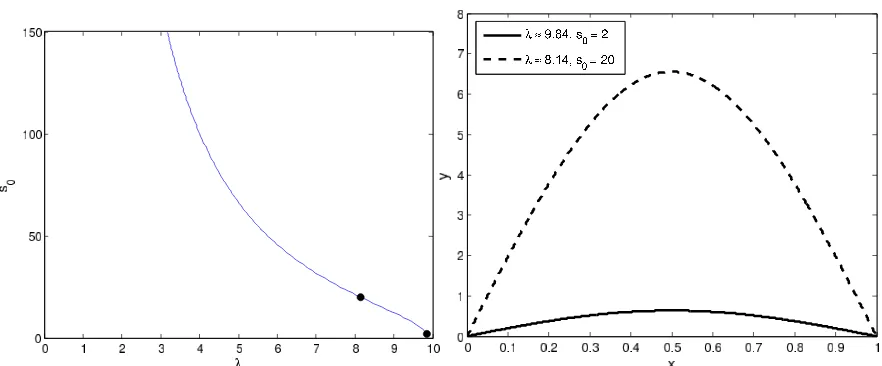
The lemma above gives some indication of the complex interplay between s0 and λ (which are also connected withkyk), and the numerical resolution of (14)-(15) provides a convenient means to visualize that relationship. The graph on the left in Figure 1 shows a curve in the (λ, s0)-plane for which solutions of (14)-(15) exist. The value of
kyk is monotonic increasing along this curve moving from left to right. Notice that for a given value of y′(0) =s
Figure 1: (left) A curve in the (λ, s0)-plane for which (14)-(15) has a positive solution. (right) The solutions corresponding to the two points highlighted in the graph on the left. For both solutions y′(0) = s
0 ≈ 1.5, so they share the same slope at the left boundary. However the value of kyk is obviously different for each, and in fact they also correspond to different eigenvalues λ.
of Figure 1 and the corresponding solutions of (14)-(15) for those values of s0 and λ are shown in the right graph.
The spectrum shown on the left in Figure 1 corresponds to the first mode. The solutions ycorresponding to the points along the curve in the (λ, s0)-plane are positive solutions of the given semilinear SLP. With further analysis we can describe similar curves in the (λ, s0)-plane corresponding to higher modes, none of which are positive solutions. We note in passing that the (λ, s0)-curve for one mode intersects the (λ, s0 )-curve for the next highest mode.
Finally, the solutions in the right graph of Figure 1 fit well with the asymptotic results of Lemma 3.1. In particular, the maximum of each eigenfunction is easily observed to be in line with the estimates given above.
4
Autonomous SLP (Approximation
L
≈
L
A)
We consider the autonomous SLP
LA(y, λ) =y′′+λy+ǫλ3y3 = 0, x∈(0,1), (21)
y(0) =y(1) = 0 (22)
following mostly the approach used by Graef et al. in [1, 2], where almost the same SLP is considered. We introduce the Liapunov function for this model
L = (y′) 2 2 +λ
y2 2 +ǫλ
3y4
Then using the first of the boundary conditions in (22) and y′(0) =s
The following results follow from a similar analysis in [1, 2].
Lemma 4.1
(i) The first eigenfunction of SLP (21)-(22) has a single maximum atx= 1 2, y
We may directly combine the results above into a single relation for y′ as follows
y′ =±√λp
Equations (25) and (27) give a parametric representation of the (λ, s0)-dependence that we seek. The parameter ˆy2 may be eliminated to produce a single implicit relation between λ and s0. For the lemma below, recall that the positive solutions we seek require s0 >0.
To prove (ii) we first estimate the denominator of the left hand side of (27). The inequality 0≤sin2(θ)≤1 implies the following inclusion
or after simplification
which immediately implies that λ < π2. Equation (25) implies that
ǫλ2yˆ2 =−1 +
q
1 + 2ǫλs2
0. (29)
Combining (28) and (29) yields the inclusion
π2−λ
0 is bounded above which implies
λ ∼ π2 and hence π2−λ ∼ s2
0 . This establishes all of (ii). Finally letting s0 → 0 in (25) and using (ii) immediately implies (iii). This com-pletes the proof.
We note the similarity between the estimates for the maximum of the first mode, ˆ
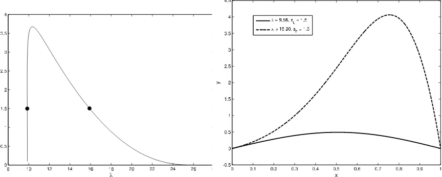
y, given for the semilinear problem in Section 3 and here for the autonomous problem. As with the semilinear problem, a numerical treatment fills in the part of the curve in the (λ, s0)-plane between the limiting cases described by the asymptotic results of Lemma 4.2. Using the fixed value ǫ = 10−4 and an approach similar to the one described in Section 3, numerical solutions to the autonomous SLP (21)-(22) can be found. The corresponding (λ, s0)-curve is shown in Figure 2. We note that for each
s0 > 0 there exists a unique λ on the spectrum for the autonomous SLP (21)-(22). This is not the case for the other two models – semilinear and fully nonlinear – that we consider in this work.
5
Fully Nonlinear SLP (Operator
L)
We consider the SLP
L(y, λ) =y′′− kyk2y′+λy+ǫλ3y3 = 0, x∈(0,1), (31)
y(0) =y(1) = 0. (32)
The Liapunov function for the SLP above is
Figure 2: (left) The curve in the (λ, s0)-plane for which (21)-(22) has a positive solution. (right) The solutions corresponding to the two points shown in the graph on the left.
and along with the slope s0 =y′(0) we obtain (y′)2 −2kyk2
Z x
0
(y′)2dη+λy2+ǫλ 3 2 y
4 =s2
0. (34)
This last identity, evaluated at x= 1 and using s1 =y′(1), yields
s21−2kyk2ky′k2 =s20. (35)
For the point where the first eigenfunction has a maximum, (ˆx,yˆ), identity (34) allows us to obtain
λyˆ2+ ǫλ 3 2 yˆ
4 =s2
0+ 2kyk2ky′k2. (36) We also introduce the following SLP
L(y, λ) =y′′+kyk2y′+λy+ǫλ3y3 = 0, x∈(0,1), (37)
y(0) =y(1) = 0 (38)
which is similar to (31)-(32), differing only in the sign of the first-order term.
Some properties of the first eigenfunctions for (31)-(32), as well as (37)-(38), are given by the following Lemma.
Lemma 5.1
(i)
s0 <|s1| < s0ekyk 2
. (39)
(ii)
Proof. The first of the inequalities, i.e. s0 < |s1|, follows immediately from (35). Denotingz(x) = (y′)2
which may be reduced to the Cauchy problem
z′(x)−2kyk2z(x) =f′(x), z(0) =s20(=f(0)). (44) The solution of this Cauchy problem is found in the standard way. Integrating by parts and utilizing the definition of f(x) in the expression for the solution, we obtain
z(x) = s20e2kyk2x+ evaluating the first term in the integral, and estimating two other terms by zero yields
s21 = s20e2kyk2 −2kyk2
This establishes the right half of (i).
To prove inequality (ii) above, we subtract (35) from (34) to find
(y′)2 =s21−
The left-hand side of (iii) immediately follows from (36) and the very same identity along with (35) further shows that
Figure 3: (left) A curve in the (λ, s0)-plane for which (31)-(32) has a positive solution. (right) The solutions corresponding to the two points shown in the graph on the left.
completing the right-hand side of (iii).
We finally observe that the substitution of ¯x = 1−x transforms (31)-(32) into (37)-(38). This completes the proof.
We note that for the autonomous SLP (21)-(22) the inequalities in (i) and (iii) of the lemma above become equalities. (See Section 4.)
For the semilinear SLP (14)-(15) all statements of Lemma 5.1 remain the same if we let ǫ = 0. Yet for the semilinear SLP we may sharpen (39) into
|s1|=s0e 1 2kyk
2
.
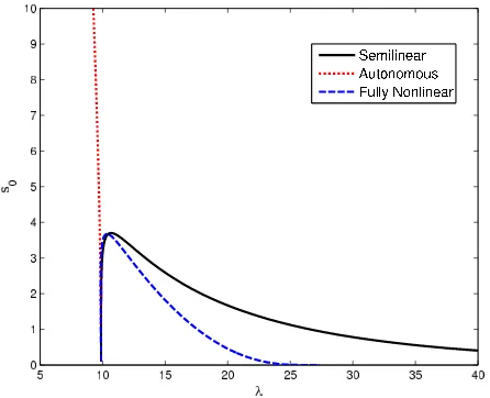
As with the semilinear model of Section 3 and the autonomous model of Section 4, we obtain numerical solutions to the fully nonlinear SLP (31)-(32) using a similar numerical technique. The first mode of the spectrum of the fully nonlinear SLP and two particular solutions are shown in Figure 3.
Figure 4: Each of the three models – semilinear, autonomous, and fully nonlinear – has a distinct first mode. All agree near (π2,0).
6
Unsolved Problems
There are two unsolved problems that the authors would like to briefly mention in connection with the fully nonlinear SLP, (31)-(32).
Problem 6.1 –The(λ, s0)-dependence for the fully nonlinear SLP (31)-(32) has been
studied numerically. How can the same problem be tackled analytically?
Moreover, if we temporarily assume kyk to be known, we may invert the linear (actually semilinear) operatorLand reduce the SLP (31)-(32) to the following integral equation,
y(x) =ǫλ3
Z 1
0
K(x, t,kyk, λ)y3(t)dt (45)
where the kernel K has the following representation
K(x, t,kyk, λ) = K1(x,kyk, λ)
K1(1,kyk, λ)
K1(1−t,kyk, λ)−K1(x−t,kyk, λ)χ(0,x)(t),
K1(x,kyk, λ) = 1 2πi
Z
C
epx 1
p2− kyk2p+λdp,
with χ(0,x)(t) the characteristic function and C the standard contour in the complex plane that appears in the Laplace transform. So more specifically, Problem 6.1 has the the form
point theorem [6, 5, 7]?
The SLP for the nonlinear differential equation
y′′+q(x)y+λ[a(x)−f(x, y, y′)]y= 0, x∈(0,1) (46)
subject to standard BC is studied in a series of papers [10, 11]. It is assumed there that
f(x, ξ, η)≥0 (47)
for x∈[0,1], 0<|ξ|,|η|< ρfor some constant ρ >0. The dependence (λ, j), where j
is the number of zeros of the corresponding eigenfunction, is studied extensively. Scaling y(x) in the autonomous SLP (21)-(22) (see [1, 2]) yields the ODE
y′′+λ
1 + 2y2
y = 0 (48)
so that f(x, ξ, η) =−2ξ2 which obviously fails to satisfy the requirement (47).
Problem 6.2–Is it possible to develop the results of the current paper in terms of the (λ, j)-dependence?
7
Conclusion
We have studied analytically and numerically three Sturm-Liouville problems. The main SLP is fully nonlinear and nonlocal and has a structure similar to the SLP which describes the stability of a wing (or panel) in an airflow. In that case, the spectral parameterλis proportional to the Mach number. Two other Sturm-Liouville problems represent simplifications of the main model, in particular when we neglect either the nonlocal term or the higher order nonlinear term. Some information about the first eigenfunction y(x) and the corresponding curve (λ, s0) is presented (where s0 is the slope ofy(x) at one endpoint). It is established to what extent the two approximations of the main model produce similar (λ, s0)-dependencies. A robust numerical simulation is used to illuminate in detail the parts of the spectrum between the limiting cases given in the asymptotic analyses.
8
Acknowledgment
The authors thank the referee for the contribution of many helpful remarks while revising this manuscript.
References
[1] B. P. Belinskiy, J. R. Graef and R. E. Melnik, The stability of a wing in a flow, Neural, Parallel & Scientific Computations 14 (2006), 75-96.
[2] B. P. Belinskiy, J. R. Graef and R. E. Melnik, Modeling a wing in an air flow, Colloquium on Differential and Difference Equations CDDE 2006 Proceedings (O. Dosly and P. Rehak, Editors) Folia FSN Universitatis Masarykianae Brunensis, Mathematica 16 (2007), 21-31.
[3] V. V. Bolotin, Nonconservative Problems of the Theory of Elastic Stability, Perg-amon Press, New York, 1963.
[4] A. Erdelyi, Asymptotic Expansions, Dover Press, USA, 1956.
[5] J. R. Graef and B. Yang, Boundary value problems for second order nonlinear ordinary differential equations, Comm. Appl. Anal. 6 (2002), 273-288.
[6] J. Henderson and H. Wang, Positive solutions for nonlinear eigenvalue problems, J. Math. Anal. Appl. 208 (1997), 252-259.
[7] M. A. Krasnosel’skii,Positive Solutions of Operator Equations, Noordhoff, Gronin-gen, 1964.
[8] L. Librescu, P. Marzocca and W. A. Silva, Linear/nonlinear supersonic panel flutter in a high-temperature field, Journal of Aircraft41 (4) (2004), 918-924.
[9] L. Librescu, P. Marzocca and W. A. Silva, Supersonic/hypersonic flutter and post-flutter of geometrically imperfect circular cylindrical panels, Journal of Spacecraft and Rockets 39 (5) (2002), 802-812.
[10] J. W. Macki and P. Waltman, A nonlinear boundary value problem of Sturm-Liouville type for a two-dimensional system of ordinary differential equations, SIAM J. Appl. Math. 21 (1971), 225-231.
[11] J. W. Macki and P. Waltman, A nonlinear Sturm-Liouville problem,Indiana Uni-versity Mathematics Journal 22 (3) (1972), 217-225.