23 11
Article 05.3.8
Journal of Integer Sequences, Vol. 8 (2005), 2
3 6 1 47
The Descent Set and Connectivity Set of a
Permutation
Richard P. Stanley
1Department of Mathematics
Massachusetts Institute of Technology
Cambridge, MA 02139
USA
[email protected]
Abstract
The descent set D(w) of a permutation w of 1,2, . . . , n is a standard and well-studied statistic. We introduce a new statistic, the connectivity set C(w), and show that it is a kind of dual object toD(w). The duality is stated in terms of the inverse of a matrix that records the joint distribution ofD(w) andC(w). We also give a variation involving permutations of a multiset and aq-analogue that keeps track of the number of inversions ofw.
1
A duality between descents and connectivity.
Let Sn denote the symmetric group of permutations of [n] = {1,2, . . . , n}, and let w =
a1a2· · ·an∈Sn. The descent set D(w) is defined by
D(w) ={i : ai > ai+1} ⊆[n−1].
The descent set is a well-known and much studied statistic on permutations with many applications, e.g., [6, Exam. 2.24, Thm. 3.12.1][7, §7.23]. Now define the connectivity set
C(w) by
C(w) ={i : aj < ak for all j ≤i < k} ⊆[n−1]. (1)
The connectivity set seems not to have been considered before except for equivalent defini-tions by Comtet [3, Exer. VI.14] and Callan [1] with no further development. H. Wilf has pointed out to me that the set of splitters of a permutation arising in the algorithm Quicksort
[8, §2.2] coincides with the connectivity set. Some notions related to the connectivity set have been investigated. In particular, a permutationwwithC(w) =∅ is calledconnected or
indecomposable. If f(n) denotes the number of connected permutations in Sn, then Comtet
[3, Exer. VI.14] showed that
X
n≥1
f(n)xn= 1− 1
P
n≥0n!xn
,
and he also considered the number #C(w) of components. He also obtained [2][3, Exer. VII.16] the complete asymptotic expansion of f(n). For further references on connected permuta-tions, see Sloane [4]. In this paper we will establish a kind of “duality” between descent sets and connectivity sets.
We write S = {i1, . . . , ik}< to denote that S = {i1, . . . , ik} and i1 < · · · < ik. Given
S ={i1, . . . , ik}< ⊆[n−1], define
η(S) =i1! (i2−i1)!· · ·(ik−ik−1)! (n−ik)!.
Note thatη(S) depends not only on S but also onn. The integern will always be clear from the context. The first indication of a duality between C and D is the following result.
Proposition 1.1. Let S ⊆[n−1]. Then
#{w∈Sn : S ⊆C(w)} = η(S)
#{w∈Sn : S ⊇D(w)} = n!
η(S).
Proof. The result forD(w) is well-known, e.g., [6, Prop. 1.3.11]. To obtain a permutation
wsatisfyingS⊇D(w), choose an ordered partition (A1, . . . , Ak+1) of [n] with #Aj =ij−ij−1
(withi0 = 0, ik+1=n) inn!/η(S) ways, then arrange the elements of A1 in increasing order,
followed by the elements of A2 in increasing order, etc.
Similarly, to obtain a permutation w satisfying S ⊆ C(w), choose a permutation of [i1]
in i1! ways, followed by a permutation of [i1 + 1, i2] := {i1+ 1, i1 + 2, . . . , i2} in (i2 −i1)!
ways, etc. ✷
Let S, T ⊆[n−1]. Our main interest is in the joint distribution of the statistics C and
D, i.e., in the numbers
XST = #{w∈Sn : C(w) = S, D(w) = T},
whereS = [n−1]−S. (It will be more notationally convenient to use this definition ofXST
rather than having C(w) =S.) To this end, define
ZST = #{w∈Sn : S ⊆C(w), T ⊆D(w)}
= X
S′⊇S T′⊇T
XS′T′. (2)
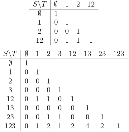
For instance, if n = 4, S = {2,3}, and T = {3}, then ZST = 3, corresponding to the
permutations 1243, 1342, 1432, while XST = 1, corresponding to 1342. Tables of XST for
S\T ∅ 1 2 12
∅ 1
1 0 1
2 0 0 1
12 0 1 1 1
S\T ∅ 1 2 3 12 13 23 123
∅ 1
1 0 1
2 0 0 1
3 0 0 0 1
12 0 1 1 0 1
13 0 0 0 0 0 1
23 0 0 1 1 0 0 1
123 0 1 2 1 2 4 2 1
Figure 1: Table of XST for n = 3 andn = 4
S\T ∅ 1 2 3 4 12 13 14 23 24 34 123 124 134 234 1234
∅ 1
1 0 1
2 0 0 1
3 0 0 0 1
4 0 0 0 0 1
12 0 1 1 0 0 1
13 0 0 0 0 0 0 1
14 0 0 0 0 0 0 0 1
23 0 0 1 1 0 0 0 0 1
24 0 0 0 0 0 0 0 0 0 1
34 0 0 0 1 1 0 0 0 0 0 1
123 0 1 2 1 0 2 4 0 2 0 0 1
124 0 0 0 0 0 0 0 1 0 1 0 0 1
134 0 0 0 0 0 0 1 1 0 0 0 0 0 1
234 0 0 1 2 1 0 0 0 2 4 2 0 0 0 1
1234 0 1 3 3 1 3 10 8 6 10 3 3 8 8 3 1
Theorem 1.1. We have
ZST =
½
η(S)/η(T), if S ⊇T; 0, otherwise,
Proof. Letw=a1· · ·an ∈Sn. If i∈C(w) then ai < ai+1, soi6∈D(w). HenceZST = 0
if S 6⊇T.
Assume therefore that S ⊇ T. Let C(w) ={c1, . . . , cj}< with c0 = 0 and cj+1 =n. Fix
0≤h ≤j, and let
[ch, ch+1]∩T ={ch =i1, i2, . . . , ik =ch+1}<.
Ifw=a1· · ·an with S ⊆C(w) andT ⊆D(w), then the number of choices forach+ 1, ach+
2, . . . , ach+1 is just the multinomial coefficient
µ
ch+1−ch
i2−i1, i3−i2, . . . , ik−ik−1
¶
:= (ch+1−ch)!
(i2 −i1)! (i3−i2)!· · ·(ik−ik−1)!
.
Taking the product over all 0≤h≤j yields η(S)/η(T). ✷
Theorem 1.1 can be restated matrix-theoretically. Let M = (MST) be the matrix whose
rows and columns are indexed by subsets S, T ⊆[n−1] (taken in some order), with
MST =
½
1, if S ⊇T; 0, otherwise.
Let D = (DST) be the diagonal matrix with DSS = η(S). Let Z = (ZST), i.e., the
ma-trix whose (S, T)-entry is ZST as defined in (2). Then it is straightforward to check that
Theorem 1.1 can be restated as follows:
Z =DM D−1. (3)
Similarly, let X = (XST). Then it is immediate from equations (2) and (3) that
M XM =Z. (4)
The main result of this section (Theorem1.2below) computes the inverse of the matrices
X,Z, and a matrixY = (YST) intermediate between X and Z. Namely, define
YST = #{w∈Sn : S ⊆C(w), T =D(w)}. (5)
It is immediate from the definition of matrix multiplication and (4) that the matrixY satisfies
Y =M X =ZM−1. (6)
In view of equations (3), (4) and (6) the computation of Z−1, Y−1, and X−1 will reduce
to computing M−1, which is a simple and well-known result. For any invertible matrix
N = (NST), write NST−1 for the (S, T)-entry ofN
−1.
Lemma 1.1. We have
M−1
ST = (−1)
#S+#TM
Proof. Let f, g be functions from subsets of [n] to R (say) related by
f(S) = X
T⊆S
g(T). (8)
Equation (7) is then equivalent to the inversion formula
g(S) = X
T⊆S
(−1)#(S−T)f(T). (9)
This is a standard combinatorial result with many proofs, e.g., [6, Thm. 2.1.1, Exam. 3.8.3]. ✷
Theorem 1.2. The matrices Z, Y, X have the following inverses:
Z−1
Equation (10) is then an immediate consequence of Lemma 1.1 and the definition of matrix multiplication.
Equation (11) is now an immediate consequence of the Principle of Inclusion-Exclusion (or of the equivalence of equations (8) and (9)). Equation (12) is proved analogously to (11) using X−1 =Y−1M. ✷
Note. The matrix M represents the zeta function of the boolean algebra Bn [6, §3.6]. Hence Lemma 1.1 can be regarded as the determination of the M¨obius function of Bn [6,
Exam. 3.8.3]. All our results can easily be formulated in terms of the incidence algebra of
Bn.
Note. The matrixY arose from the theory of quasisymmetric functions in response to a
Let Comp(n) denote the set of all compositions α = (α1, . . . , αk) of n, i.e, αi ≥ 1 and
P
αi = n. Let α = (α1, . . . , αk) ∈ Comp(n), and let Sα denote the subgroup of Sn
consisting of all permutations w = a1· · ·an such that {1, . . . , α1} = {a1, . . . , aα1}, {α1 +
1, . . . , α1 +α2} ={aα1+1, . . . , aα1+α2}, etc. Thus Sα ∼=Sα1 × · · · ×Sαk and #Sα =η(S),
where S = {α1, α1 +α2, . . . , α1 +· · ·+αk−1}. If w ∈ Sn and D(w) = {i1, . . . , ik}<, then
define the descent composition co(w) by
co(w) = (i1, i2−i1, . . . , ik−ik−1, n−ik)∈Comp(n).
LetLα denote the fundamental quasisymmetric function indexed byα[7, (7.89)], and define
Rα =
X
w∈Sα
Lco(w). (13)
Given α = (α1, . . . , αk)∈ Comp(n), letSα ={α1, α1+α2, . . . , α1+· · ·+αk−1}. Note that
w∈Sα if and only if Sα ⊆C(w). Hence equation (13) can be rewritten as
Rα =
X
β
YSαSβLβ,
with YSαSβ as in (5). It follows from (5) that the transition matrix between the bases Lα
andRα is lower unitriangular (with respect to a suitable ordering of the rows and columns).
Thus the set {Rα : α ∈Comp(n)} is a Z-basis for the additive group of all homogeneous
quasisymmetric functions over Z of degreen. Moreover, the problem of expressing the Lβ’s
as linear combinations of the Rα’s is equivalent to inverting the matrixY = (YST).
The question of Billera and Reiner mentioned above is the following. Let P be a finite poset, and define the quasisymmetric function
KP =
X
f
xf,
where f ranges over all order-preserving maps f : P → {1,2, . . .} and xf =Q
t∈P xf(t) (see
[7, (7.92)]). Billera and Reiner asked whether the quasisymmetric functions KP generate
(as aZ-algebra) or even span (as an additive abelian group) the space of all quasisymmetric functions. Let m denote an m-element antichain. The ordinal sum P ⊕Q of two posets
P, Q with disjoint elements is the poset on the union of their elements satisfying s ≤ t if either (1) s, t ∈ P and s ≤t in P, (2) s, t ∈ Q and s ≤t in Q, or (3) s ∈ P and t ∈Q. If
α= (α1, . . . , αk)∈Comp(n) then letPα =α1⊕ · · · ⊕αk. It is easy to see thatKPα =Rα, so
theKPα’s form aZ-basis for the homogeneous quasisymmetric functions of degreen, thereby
answering the question of Billera and Reiner.
2
Multisets and inversions.
Let T ={i1, . . . , ik}< ⊆[n−1]. Define the multiset
Proof. The equality of the three expressions on the right-hand side is clear, so we need only show that
#{w∈SNT : C(w) = S}= #{w∈Sn : C(w) =S, D(w)⊇T}. (14)
Let T = {i1, . . . , ik}< ⊆ [n−1]. Given w ∈ Sn with C(w) = S and D(w) ⊇ T, in w−1
replace 1,2, . . . , i1 with 1’s, replace i1 + 1, . . . , i2 with 2’s, etc. It is easy to check that this
yields a bijection between the sets appearing on the two sides of (14). ✷
Theorem 2.1. We have
Z(q)ST =
½
qz(T)η(S, q)/η(T , q), if S∩T =∅;
0, otherwise.
Proof. Preserve the notation from the proof of Theorem 1.1. If (s, t) is an inversion of w (i.e., s < t and as > at) then for some 0 ≤ h ≤ j we have ch + 1 ≤ s < t ≤ ch+1.
It is a standard fact of enumerative combinatorics (e.g., [5, (21)][6, Prop. 1.3.17]) that if
U ={u1, . . . , ur}< ⊆[m−1] then
Hence we can parallel the proof of Theorem 1.1, except instead of merely counting the number of choices for the sequence u= (ach, ach+ 1, . . . , ach+1) we can weight this choice by
The proof now is identical to that of Theorem 1.2. ✷
3
Acknowledgments
I am grateful to the referee for several suggestions that have enhanced the readability of this paper.
References
[1] D. Callan, Counting stabilized-interval-free permutations, J. Integer Sequences (elec-tronic) 7 (2004), Article 04.1.8.
[2] L. Comtet, Sur les coefficients de l’inverse de la s´erie formelle P
n!tn, Comptes Rend.
Acad. Sci. Paris,A 275 (1972), 569–572.
[3] L. Comtet,Advanced Combinatorics, Reidel, 1974.
[4] N. J. A. Sloane, The On-Line Encyclopedia of Integer Sequences, sequenceA003319.
[5] R. Stanley, Binomial posets, M¨obius inversion, and permutation enumeration, J. Com-binatorial Theory (A) 20 (1976), 336–356.
[6] R. Stanley, Enumerative Combinatorics, vol. 1, Wadsworth and Brooks/Cole, 1986; sec-ond printing, Cambridge University Press, 1996.
[7] R. Stanley, Enumerative Combinatorics, vol. 2, Cambridge University Press, 1999.
[8] H. Wilf, Algorithms and Complexity, second ed., A K Peters, 2002.
2000 Mathematics Subject Classification: Primary 05A05.
Keywords: descent set, connected permutation, connectivity set.
(Concerned with sequence A003319.)
Received July 18 2005; revised version received August 16 2005. Published in Journal of Integer Sequences, August 24 2005.