Constructing Soliton and Kink Solutions
of PDE Models in Transport and Biology
Vsevolod A. VLADIMIROV, Ekaterina V. KUTAFINA and Anna PUDE LKO Faculty of Applied Mathematics AGH University of Science and Technology, Al. Mickiewicza 30, 30-059 Krak´ow, Poland
E-mail: [email protected], [email protected]
Received November 30, 2005, in final form May 24, 2006; Published online June 19, 2006 Original article is available athttp://www.emis.de/journals/SIGMA/2006/Paper061/
Abstract. We present a review of our recent works directed towards discovery of a periodic, kink-like and soliton-like travelling wave solutions within the models of transport phenomena and the mathematical biology. Analytical description of these wave patterns is carried out by means of our modification of the direct algebraic balance method. In the case when the analytical description fails, we propose to approximate invariant travelling wave solutions by means of an infinite series of exponential functions. The effectiveness of the method of approximation is demonstrated on a hyperbolic modification of Burgers equation.
Key words: generalized Burgers equation; telegraph equation; model of somitogenesis; direct algebraic balance method; periodic and solution-like travelling wave solutions; approxima-tion of the soliton-like soluapproxima-tions
2000 Mathematics Subject Classification: 35C99; 34C60; 74J35
1
Introduction
It is well known that methods of obtaining general solutions for the majority of nonlinear evo-lutionary PDEs actually do not exist. The already known methods of integration, such as the inverse scattering technique, are applied merely to so called completely integrable equations [1]. These equations form a very important but relatively small family, which does not include e.g. nonlinear dissipative models, describing the spatio-temporal patterns formation and evolu-tion [2]. One of the few alternatives to numerical methods of the investigations of those models that are not completely integrable are the symmetry methods [3,4] which are effective when the system under consideration admits a non-trivial group of transformations. Yet, these methods cannot be treated as universal tools for obtaining analytical solutions. In fact, the self-similar reduction, when applied to a nonlinear PDE, gives another nonlinear differential equation with a fewer number of independent variables and it is difficult to expect that the procedure will lead to quadratures in every particular case. Obviously the chances to obtain this way the analytical description of solutions with the required properties and asymptotic behavior (such as e.g. periodic, kink-like or soliton-like travelling wave solutions) are, generally speaking, very small.
investigate the influence of small addends upon the stability and the evolution properties of the invariant solutions.
Compared to classical symmetry methods, more powerful tools for finding out solutions with the given properties, can be provided by so-called direct algebraic balance method, based upon representing solutions in the form of rational algebraic combinations of properly chosen functions, closed with respect to the algebraic operations and differentiation [7,8,9,10]. However, within this method one must solve, as a rule, very large systems of nonlinear algebraic equations. Regardless of this purely technical reason, the ansatz-based method cannot be treated as the remedy, because there are known evolution PDEs which possess analytical solutions that cannot be obtained, at least, within a particular set of elementary functions (hyperbolic, trigonometric, polynomial, etc.). And it is rather doubtful that a fully universal ansatz for finding out the analytical solutions to nonlinear PDEs can ever be found. Nevertheless, it is possible to answer the question of whether the solution of this or that sort does exist within the given set of invariant solutions, whenever the procedure of a self-similar reduction leads to the system of autonomous ODEs. And in the situation when the direct algebraic balance method, based on the representing solution we are looking for in the form of finite combination of the given functions fails, we propose to express it by means of the infinite series.
The aim of this study is to review our recent work directed towards the description of the already mentioned wave patterns, i.e. the kink-like and soliton-like travelling wave solutions, in various non-local models, simulating the transport phenomena. In our earlier work we in-vestigated merely the set of travelling wave (TW) solutions, being invariant with respect to the group of the spatio-temporal translations, nevertheless, systems obtained via the symmetry reduction prove to be sufficiently difficult to analyze and solve exactly. Therefore we use a complex approach including a qualitative analysis, our own interpretation of the ansatz-based method and approximation of the invariant solutions by means of infinite series of exponential functions.
The structure of the article is as follows. In Section 2 we present a certain modification of the direct algebraic method, put forward in papers [7, 8, 9]. Employing this modification we obtain the kink-like and soliton-like TW solutions for the hyperbolic modification of Burgers equation, telegraph equation, nonlinear d’Alembert equation and the somitogenesis model. In Section 3 we present the results of a qualitative investigations of a set of TW solutions for the hyperbolic modification of Burgers equation. It demonstrates the existence of the TW solution-like solutions, yet these solutions cannot be described by the finite algebraic combination of elementary functions. Therefore we propose to approximate the invariant solitary wave solutions by an infinite series of the exponential functions.
2
Exact soliton-like and kink-like solutions
for transport equations
2.1 Modif ication of the direct algebraic method and its applications
The essence of theunified direct algebraic methodin E. Fan’s paper [7], is based on the observation that particular solutions of any system of PDE’s
Hν ui, uit, uix, uixx, . . .
= 0, i= 1,2, . . . , m, ν= 1,2, . . . , n (1)
which do not depend on (t, x) coordinates in explicit form, can be presented as a polynomial expansion
ui(ξ) = s
X
µ=0
where aµ are unknown parameters, while functionφ(ξ) satisfies the equation
Note that in order to obtain non-trivial solutions, one should “balance” the numbers r and s (for details see [7]).
Depending on the conditions posed on the parameters cν, solutions to the equation (3) are expressed by elliptic Jacobi functions, and in particular cases by hyperbolic or trigonometric functions [7]. The properties of these functions are inherited by the solution of the initial system which can be presented in the form (2). In fact this methodology is constructive and algorithmic if the functions Hν(·,·, . . .) arising in (1) are algebraic or rational ones. With this assumption, for any set of functions
ui mi=1 that can be represented as (2), the LHS of the equations (1) can be presented in the form of finite linear combinations of functions φk(ξ) and φl(ξ) ˙φ(ξ), k, l= 0,1,2, . . .:
When equating to zero all the coefficients of these decompositions, one obtains a system of non-linear algebraic equations, that determine the particular solutions of the initial system of PDE’s (for more details see [7]). It must be stressed that the method does not guarantee obtaining of the general solution, even within the set (2), for its effectiveness depends on one’s ability to solve a system of nonlinear algebraic equations. On the other hand, it enables calculation of particular solutions possessing some predictable properties.
An enforced version of Fan’s method was put forward recently in [8, 9]. It was used for determining of exact solutions of the equation
ut+Auux−κuxx=f(u).
More precisely, the following ansatz was proposed:
u=
nation, the multi-parameter families of the exact solutions were obtained in the situation when the pure form of Fan’s methodology does not work [8].
On analyzing different versions of the ansatz-based method, one can conclude that effective-ness of their employment is based on the mere fact that the family of functionsφµ(ξ) andφνφ˙(ξ) is closed with respect to the algebraic operations and differentiation. In view of this, a quite natural generalization of the already mentioned ansatzes can be as follows:
u= f(ξ)
2.2 Soliton-like and kink-like TW solutions for the generalized transport equations
Let us consider the following equations:
τ utt+Auux+But−κuxx =f(u) =
X
ν∈I
λνuν, (6)
whereτ,A,B,κare non-negative constants. ForA= 0 equation (6) coincides with the nonlinear telegraph equation; forA6= 0 it coincides with the hyperbolic generalization of Burgers equation, while for A =B = 0 – with the nonlinear d’Alembert equation. The hyperbolic modifications of nonlinear transport equations arise naturally when the effects of temporal non-locality are taken into account [11].
Assuming that the solitons and kinks can be expressed by powers of function sech(ξ), which is the particular solution of equation (3) and function sinh(ξ) which appears in the odd derivatives of the function sech(ξ), we use the following ansatz:
u(ξ) = f(ξ)
Inserting the ansatz (7) ( or (8)) into (6) and executing all the necessary operations, we obtain an algebraic equation containing, respectively, functions sechµ(αξ), sechν(αξ) sinh(αξ) or exp [µαξ]. Deeming them functionally independent and equating to zero the corresponding coefficients, we go to the system of algebraic equations. We do not demonstrate the details of these calculations since they are simple but cumbersome. The calculations were performed through the aid of a software application “Mathematica”. The results obtained are presented below.
satisfies equation (6) if the following conditions hold:
do whenα = 2√−λ0λ2/v,a0 =−a1= Another example of the kink-like solution defined by the formulae (9), (10) is as follows:
u(t, x) = 2
satisfies the equation (6) providing that the following conditions hold:
λ0= 2a20a12αh/∆2, λ1/2 =−2a0a1α(3hΘ +Bv∆)/∆2,
3+κ)/τ . This solution is always singular, because for arbitrary values of the parameters the expression in the denominator of the formula (11) vanishes for some ξ ∈R.
satisfies equation (6) when the following conditions hold:
λ1= ((a21b20+ 4a0a1b0b1+a20(−6b20+b21))αh/∆2,
λ2= 3b0(2a0b20−a1b0b1−a0b21)αh/∆2, λ3 =−2b0(b20−b21)αh/∆2. (13)
For a0 6= 0, b0 6= 0, |a1|+|b1| 6= 0 equation (12) defines the soliton-like solution. One of the parameters contained in (12) can be chosen arbitrarily, while the rest can be expressed, using (13), as the functions of the parameters, defining equation (6). We omit doing this in the general case, but present one particular example. Thus, for b1 = 0, b0 = 1 and arbitrary α we have the solution
u(t, x) = a0+ 2a1e
α(x+vt)+a
0e2α(x+vt) 1 +e2α(x+vt) , with
a0=−λ2/(3λ3), a1 =
q
2(λ22−λ1λ3)/λ23, v =±
q
λ1−λ22/(3λ3) +κα2/(τ α2),
and the additional conditionλ0+λ1a0+λ2a20+λ3a30 = 0. VIb. Forf(u) =λ1/2u(t, x)1/2+λ
1u(t, x) +λ3/2u(t, x)3/2+λ2u(t, x)2 we obtain a soliton-like solution
u(t, x) = (e
α(x+vt)+ 1)4
(b0e2α(x+vt)+ (2b0+ 4b1)eα(x+vt)+b0)2 with
λ1/2 =−3αh/b1, λ1 = (12b0+ 4b1)αh/b1,
λ3/2 =−(15b20+ 10b0b1)αh/b1, λ2= (6b20b1+ 6b30)αh/b1.
VIc. Forf(u) =λ0+λ1/2u(t, x)
1
2 +λ1u(t, x) +λ3/2u(t, x) 3
2 a localized wave packet
u(t, x) = (a0e
2α(x+vt)+ (2a
0+ 4a1)eα(x+vt)+a0)2 (eα(x+vt)+ 1)4
defines a solution of (6) if the following conditions hold:
λ0= 2a20(a0+a1)αh/a1, λ1/2 = (9a20+ 6a0a1)αh/a1, λ1= (12a0+ 4a1)αh/a1, λ3/2=−5αh/a1.
VId. Forf(u) =λ1u(t, x) +λ3/2u(t, x)
3
2 +λ2u(t, x)2 the function
u(t, x) = 4e
2α(x+vt)
(a0e2α(x+vt)+ 2a1eα(x+vt)+a0)2 with
λ1= 4αh, λ3/2 =−10a1αh, λ2 = (6a21−6a20)αh defines a soliton-like solution of the equation (6).
VIe. Finally, let us consider the equation
τ utt−κuxx =λ0+λ1u+λ2u2+λ3u3. (14) Substituting the ansatz u = φ(ξ), ξ = x +vt into the equation (14), we obtain, after one integration, the following ODE:
dφ dξ =±
p
c0+c1u+c2u2+c3u3+c4u4,
0 0.25 0.5 0.75 1 1.25 1.5 R
-0.75 -0.5 -0.25 0.25 0.5 0.75 Y
Figure 1. Phase portrait of dynamic system describing the TW solution of system (6): case IV.
(a) ifλ2=λ0 = 0, then equation (14) possesses a soliton-like solution
u(t, x) =p−2λ1/λ3sech
p
λ1/δξ
, λ1 >0, λ3 <0;
(b) ifλ0=λ2 = 0, then equation (14) possesses a kink-like solution
u(t, x) =p−λ1/λ3tanhp−λ1/(2δ)ξ, λ1 <0, λ3>0;
(c) ifλ0=λ3 = 0, then equation (14) possesses a soliton-like solution
u(t, x) =−[3λ1/(2λ2)] sech2pλ1/δξ/2, λ1>0.
More general results can be obtained using the fact that (14) corresponds to a Hhamiltonian case. Using the standard procedure, we obtain the following integral:
ξ =
Z
du
p
2H+ 2δ−1(λ
0u+λ1u2/2 +λ2u3/3 +λ3u4/4)
, (15)
whereHis the value of the Hamiltonian function on the given phase trajectory. The integral (15) can be calculated explicitly in terms of elliptic functions for different values of H and as special cases contains all the solutions obtained in part IV. An example of phase portrait for ∆ = 1, λ0= 2, λ1 =−11, λ2 = 15,and λ3=−6 is presented in Fig. 1.
2.3 A model of mathematical biology
Now we consider the following system [12]:
ut+Auux−uxx =f(u, z),
zt=g(u, z), (16)
where f(u, z),g(u, z) are given polynomials, andA is a positive constant.
Due to the fact that the system is autonomous we apply variables in a travelling wave form:
u(t, x) =V(ξ), z(t, x) =U(ξ),
where ξ=x+µt, and we reduce system (16) to the following system of ODE:
µV′
+AV V′ −V′′
=f(U, V), µU′
To simplify the computations, we restrict the family of admissible polynomials in RHS as follows:
f(U, V) =a1U+a2V +a3U V, g(U, V) =b1U+b2V +b3U V.
In order to obtain soliton- and kink-like solutions we proposed the following ansatz
U(ξ) = c1e ξ
d0+d1eξ+d2e2ξ
, V(ξ) = p1e ξ
q0+q1eξ+q2e2ξ
that shows the proper asymptotic behavior.
The following kink-like solutions were obtained:
U(ξ) = p1 q1+q2eξ
, V(ξ) = 2q1 Aq1+Aq2eξ
,
where
a1=µ−1, a2 = 0, a3 =
q1(1−µ) p1
, b1 =− Ap1µ
2q1
, b2= 0, b3= Aµ
2 .
For other family of parameters
a1=µ2−1, a2= − 2q1µ Ap1
, a3= 2q1
p1 ,
b1 =−
Ap1(µ2−1)µ 2q1
, b2=µ2, b3=−Aµ
the ansatz provides the following soliton-like solutions:
U(ξ) = 4p1q2e ξ
(q1+ 2q2eξ)2 ,
V(ξ) = 8q1q2e ξ
A(q1+ 2q2eξ)(2q2(µ−1)eξ+q1(µ−1)) .
3
Approximated soliton-like solutions
of the generalized Burgers equation
3.1 Existence of the soliton-like regimes within the set of TW solutions
We showed in the previous section that the ansatz (8) is quite effective in obtaining travel-ling wave solutions with given properties and asymptotics. Yet recently we realized that it is quite impossible to describe soliton-like solutions of the following generalization of the Burgers equation (GBE from now on):
τ utt+uux+ut−κuxx+γu(u2−z02) = 0, (17)
using the ansatz (8), which is more general than the generalized Hirota-like ansatzes employed in [8,9]. The first thing we are going to do in the situation when the ansatz-based methods fail, is to perform a qualitative study of the ODE system describing the TW solutions of the GBE and answer the question whether (and when) soliton-like solutions exist.
Inserting the ansatz u =U(ξ) =U(x+µt) into the equations (17) we obtain the second order leads us to the equation
d2U¯
0 (we omit bars over the variables in the following formulae). Let us rewrite (19) as the following system of the first order ODEs:
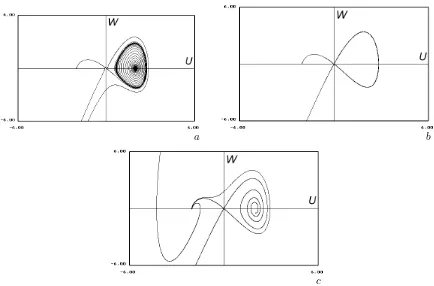
dU shows [13] that the critical point B0 is always a saddle. Depending on the values of the para-meters, two other critical points are either nodes or foci. As was declared earlier, we are looking for the homoclinic trajectory and since the dynamical system (20) is of dissipative type, this trajectory can exist only for special values of the parameters. In our attempts to capture the homoclinic loop we begin with studying the condition of the limit cycle creation in proximity of the critical point B2. If there exists a limit cycle lying in the right half plane and surrounding the critical pointB2, then its evolution in the vicinity of the unmovable saddle pointB0, caused by the change of the driven parameterµ, most probably will lead to the homoclinic bifurcation. It can be shown by inspection of the Andronov-Hopf theorem conditions and their fulfillment [14,13] that in vicinity of the critical value of the parameterµ=−1 an unstable limit cycle is created with zero radius. A further evolution of system (20) was undertaken by means of the numerical simulation in which we putA= 1. It shows that the radius of the periodic trajectory grows with the parameter µ, until the homoclinic bifurcation takes place atµ ≈ −0.836.Note that the homoclinic solution intersects the horizontal axis at the point U = x∗ ≈ 1.426095. On further growth of the parameter µ the homoclinic loop is destroyed and one of the phase trajectories starting at the unstable saddleB1reaches the critical pointB2. Patterns of the phase trajectories of system (20) obtained by means of numerical simulations are shown in Fig.2.
Thus, the homoclinic loop exists in system (20) merely at the specific values of the parameters. The construction of the approximated soliton-like solution, undertaken below is based in essential way upon the preliminary information obtained in this section.
3.2 Approximation of the soliton-like TW solution to the GBE
a b
c
Figure 2. Phase portraits of system (20); (a): µ=−0.9; (b): µ=−0.836; (c): µ=−0.8.
that gives us proper asymptotics whenξ→ ±∞. The problem is that the formula (21) does not describe the SW solution whenever m is a finite number, as it is stated below.
Lemma 1. A solitary wave solution of the equation (17)cannot be described by the formula (21). Proof . Since there is a one-to-one correspondence between the solutions of equations (18) and (19), we consider the latter one, trying to represent its homoclinic solution by means of the formula
U(T) = m
P
k=1
akexp [kαT]
1 +mP+1
r=1
brexp [rαT]
. (22)
Let us denote the numerator and denominator of the above expression by F(T), G(T) respec-tively. Inserting the ansatz (22) into the equation (19) and multiplying the resulting equation by G3, we get the expression
G(F′′
G−G′′
F) + [A(F+µG)−2G′ ](F′
G−G′
F) +F(F2−G2) = 0.
Now, gathering the coefficients standing at functions exp (αT), exp [(3m+ 2)αT] and assuming that the coefficients a1, am, bm+1 are nonzero, we obtain the following system of algebraic equations:
α2+Aµα−1 = 0, α2−Aµα−1 = 0,
Of course, the formula (22) does not give the most general expression for a solution, having the proper asymptotics at T → ±∞ and belonging to the family (8). For example, we can take the formula
instead of (22) for any natural numbersn1,n2,n3andm.But our experiments with this formula in the cases when the numerator and denominator contained, respectively, two and three terms, gave a result which is identical to that stated in Lemma1. We do not mention it here because it is too cumbersome. Concerning an expression containing more terms the result is unclear as yet, but it is rather doubtful that we would obtain a positive answer by incorporating extra terms, for a number of extra algebraic equations accompanying the “inflation” of the formula (23) exceeds in an essential way a number of extra coefficients ak,br to be determined.
So putting aside attempts to discover the analytical expression for soliton-like solutions of the GBE, we are searching for approximated solutions to the equation (19), represented by the series (24),
where x∗ is a point of intersection of the homoclinic trajectory with the horizontal axis, which, generally speaking, can be obtained from the numerical experiment. With this conditions the two branches of the homoclinic trajectory are “tied up” in the point (x∗,0).
There are two ways of determining the unknown constantsak andα. Firstly, it is possible to insert the series
into (17) and equate to zero the coefficients standing at different powers of the function exp [αT]. This way we obtain the recurrence ak+1 = ψk+1(a1, a2, . . . , ak). Another possibility is to use the initial conditions (25) and their differential consequences. As in the previous case, this approach is quite algorithmic for any second order ODE that is linear with respect to the highest derivatives. The approach is based on the following statement, which can be easily proved by means of mathematical induction.
Lemma 2. Consider the Cauchy problem U′′
(ξ) =F(ξ, U, U′
), (27)
U(0) =x0, U′(0) =x1. (28)
Suppose we are looking for the approximate solution to (27),(28) in the form U(ξ) =
N
X
k=1
Then the coefficients {ak}Nk=1 can be obtained from the conditions (28)and the N−2 equations
are recurrently expressed merely by the initial conditions x0, x1 and do not depend upon ak. So according to Lemma2, using Cauchy data (28) and their differential consequences we get the linear system
The matrix ˆMN standing at the RHS of equation (30) is of the Vandermonde type [15]. Its determinant is given by the formula
det ˆMN =α
N(N−1)
2 ·0!·1!·2!· · ·(N−1)!,
so it is always nonsingular and the system has a unique solution for each N.
Remark. The above lemma says nothing about the convergence of the series (29) to the real solution of the initial value problem (27), (28) as N → ∞. This problem needs a special investigation.
Our analysis suggests that the upper and lower branches of the homoclinic trajectory are so strongly asymmetric that the convergency of the approximated solution based on the first method of determining the coefficients of series expansions (24) takes place merely for the lower one, whereas the upper branch should be approximated with the second method only.
Thus, we approximate the lower branch of homoclinic solution by the series
ψ(T) = ∞
X
n=1
bnexp [−βT n],
truncated on a number N. The finite series is inserted into the factorized equation (19) and the coefficients standing at the subsequent powers of function exp[−βT] are equated to zero. For those values of the parameters that have been employed in the Section 2, the coefficient at {exp[−βT]}1 nullifies if β ≈0.6658. Equating to zero the coefficients of {exp[−βT]}k, we obtain the recurrence for the coefficients bk, k = 2,3, . . . , N, while b1 remains unidentified. We omit the presentation of this recurrence since it is irregular and cannot be expressed it in the analytical form. Therefore all the calculations were performed with the help of the “Mathematica” package. They were based in an essential way upon the assumption that the phase trajectory approaches the point U = x∗ = 1.426095 of the horizontal axis as T → 0. Approximate solutions corresponding to different values of the number N are shown in Fig. 3.
Figure 3. The lower branch of the homoclinic loop of system (20): numerical solution (solid) and the truncated series (24) (dashed). The coefficients ak are defined by means of the first
method. The bold dashed line is obtained for
N = 40.
Figure 4. The upper branch of the homoclinic loop of system (20): numerical solution (solid) and the truncated series (24) (dashed). The coefficients ak are defined by means of the first
method.
Figure 5. The upper branch of the homoclinic loop of system (20): numerical solution (solid) and the truncated series (24) (dashed). The coefficients ak are defined by means of the
sec-ond method. The bold dashed line correspsec-onds to N= 20.
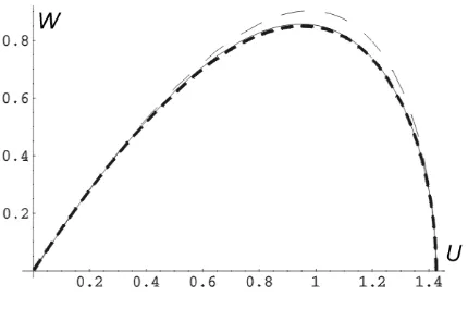
Figure 6. Solitary wave solution of equation (17) (solid) and its approximation (dashed).
we turn to the second scheme. Keeping in the series (26) N elements and substituting the truncated series into equation (19), we obtain from (25) two conditions for the coefficients ak:
U(0) = N
X
k=1
ak=x∗= 1.426095, U ′
(0) = N
X
k=1
kak = 0. (31)
The first differential consequence of these conditions gives us equation (19) itself. Taking it into the point T = 0 and employing equations (31), we obtain:
U′′ (0) =
N
X
k=1
(αk)2ak= (1−x2∗)x∗ =f3(x∗).
means of some recurrent procedure, written in “Mathematica” package. In order to obtain the parameterα, we insert the solution (26) into (19) and equate to zero the coefficientα2+Aµα−1, at the lowest power of the exponential function. For A = 1 and µ =−0.836 this gives us the value α= 1.5018.
The above procedure was used to obtain the upper branch of the homoclinic curve of sys-tem (20) (or what is the same, the left “wing” of the SW solution of the equation (19)). The results obtained are shown in Fig.5. The upper and lower branches sewed together are shown in Fig. 6, from which we can see that suggested approach quite well approximates the homoclinic solution of equation (17).
4
Concluding remarks
We have reviewed in this study the methods and tools that allow one to describe the solutions of the nonlinear PDEs with the required features and asymptotic behavior. The exact solutions presented here are obtained with the help of the ansatz (8)1, which proves to be effective when the methods described in [7,8] fail. We concentrated mainly upon the soliton-like TW solutions and their description, yet similar tools can be applied to the description of kink-like, periodic and multi-periodic solutions as well.
In contrast to the classical self-similarity methods, ansatz-based methods [7,8,9,10] enable to obtain the exact solution with required properties an asymptotics (such e.g. as the periodic, soliton-like and kink-like TW solutions). This is due to the fact that within these methods solutions are defined as algebraic combinations of certain set of functions (elementary of special ones), closed with respect to differentiation and algebraic operations, being represented in a form, enabling to control some features and the asymptotic behavior of the solutions to be described. Yet efficient employment of the direct algebraic balance methods is related to one’s ability to solve large systems of nonlinear algebraic equations. In addition to this purely technical obstacle, there is a number of evidence that none of the already known version of the balance algebraic method is fully universal. For this reason the authors put forward the method of the asymptotic description of the soliton-like TW solutions by an infinite series of exponential functions. The effectiveness of this method, connected with some general properties of the set of exponential functions [17], is demonstrated by its application to the GBE. Previous qualitative investigations showed the existence of such solutions for the specific values of the parameters and further on it was shown that these solutions cannot be described as finite algebraic combination of exponential functions.
Let us say a few words about the problem of the truncated series (24) convergence to the exact solution. A uniform convergency of a series of exponential functions to an exact solu-tion can be easily stated e.g. for the nonlinear wave equasolu-tion, because the expressions for the coefficientsanandbn are known in this case [13]. Unfortunately, for GBE the recurrent expres-sions for indices an,bn of the decomposition (24) are not known and the problem of the series convergence remains still open.
The method of approximation of solitary wave regimes, described in Section 3, is relatively easy to perform in case when the factorized system is two-dimensional. In the less trivial cases, when the factorized system is multidimensional, the homoclinic trajectories representing the soliton-like solutions become much more complicated. As an example let us mention a Shil’nikov homoclinic trajectory associated with the saddle-focus of a three-dimensional dynamical sys-tem [18, 6]. In order to deliver an approximated description of such trajectory following the methodology outlined in Section 3 of this study, it is necessary to incorporate wider class of
1During the preparation of this proof, we wre pointed to the paper [16] in which similar ansatzes were applied
functions. In earlier attempts at describing the Shil’nikov homoclinics [19], a combination of the exponential and trigonometric functions was used. The approximation employed in [19] was not very effective because of the great technical difficulties encountered. Since then a num-ber of powerful programs for the symbolic calculations were developed, and it is our hope that approximation similar to that used in [19] actually can be performed technically much more effectively.
Acknowledgments
The authors thank the anonymous referees for helpful suggestions concerning the presentation of results.
[1] Dodd R.K., Eilbek J.C., Gibbon J.D., Morris H.C., Solitons and nonlinear wave equations, London, Aca-demic Press, 1984.
[2] Glansdorf P., Prigogine I., Thermodynamics of structure, stability and fluctuations, New York, Wiley, 1971.
[3] Ovsiannikov L.V., Group analysis of differential equations, New York, Academic Press, 1982. [4] Olver P., Applications of Lie groups to differential equations, New York, Springer, 1993.
[5] Andronov A., Leontovich E., Gordon I., Maier A., Qualitative theory of second order dynamic systems, Jerusalem, Israel Program for Scientific Translations, 1971.
[6] Guckenheimer J., Holmes P., Nonlinear oscillations, dynamical systems and bifurcations of vector fields, New York, Springer, 1987.
[7] Fan E., Multiple travelling wave solutions of nonlinear evolution equations using a unified algebraic method,
J. Phys. A: Math. Gen., 2002, V.35, 6853–6872.
[8] Nikitin A., Barannyk T., Solitary waves and other solutions for nonlinear heat equations, Cent. Eur. J. Math., 2004, V.2, 840–858, math-ph/0303004.
[9] Barannyk A., Yurik I., Construction of exact solutions of diffusion equations, in Proceedings of Fifth In-ternational Conference “Symmetry in Nonlinear Mathematical Physics” (June 23–29, 2003, Kyiv), Editors A.G. Nikitin, V.M. Boyko, R.O. Popovych and I.A. Yehorchenko,Proceedings of Institute of Mathematics, Kyiv, 2004, V.50, Part 1, 29–33.
[10] Vladimirov V.A., Kutafina E.V., Exact travelling wave solutions of some nonlinear evolutionary equations,
Rep. Math. Phys., 2004, V.54, 261–271.
[11] Makarenko A.S., Mathematical modelling of memory effects influence on fast hydrodynamic and heat con-duction processes,Control and Cybernetics, 1996, V.25, 621–630.
[12] Collier J.D., McInerney D., Schnell S., Maini P.K., Gavaghan D.J., Houston P., Stern C.D., A cell cyclic model for somitogenesis: mathematical formulation and numerical simulation,J. Theor. Biol.,2000, V. 207, 305–316.
[13] Vladimirov V.A., Kutafina E.V., Toward an approximation of solitary-wave solutions of non-integrable evolutionary PDEs via symmetry and qualitative analysis,Rep. Math. Phys., 2005, V.56, 421–436.
[14] Hassard B.F., Kazarinoff N.D., Wan Y.-H., Theory and applications of the Hopf bifurcation, New York, Springer, 1981.
[15] Korn G.A., Korn T.M., Mathematical handbook, New York, McGraw-Hill, 1968.
[16] Cornille H., Gervois A., Bi-soliton solutions of a weakly nonlinear evolutionary PDEs with quadratic non-linearity,Phys. D, 1982, V.6, 1–28.
[17] Leontiev A.F., Entire functions and exponential series, Moscow, Nauka, 1983 (in Russian).
[18] Shil’nikov L.P., On one case of the existence of a countable set of periodic movements, Sov. Math. Dokl., 1965, V.6, 163–166.