E l e c t ro n ic
Jo u r n
a l o
f P
r o b
a b i l i t y
Vol. 6 (2001) Paper no. 9, pages 1–23
Journal URL
http://www.math.washington.edu/~ejpecp/ Paper URL
http://www.math.washington.edu/~ejpecp/EjpVol6/paper9.abs.html
TRANSITION DENSITY ASYMPTOTICS FOR SOME DIFFUSION PROCESSES WITH MULTI-FRACTAL STRUCTURES
Martin T. Barlow
Department of Mathematics, University of British Columbia, Vancouver, V6T 1Z2, Canada [email protected]
Takashi Kumagai
Research Institute for Mathematical Sciences, Kyoto University, Kyoto 606-8502, Japan [email protected]
AbstractWe study the asymptotics ast→0 of the transition density of a class ofµ-symmetric diffusions in the case when the measureµhas a multi-fractal structure. These diffusions include singular time changes of Brownian motion on the unit cube.
Keywordsdiffusion process, heat equation, transition density, spectral dimension, multi-fractal AMS subject classification 60J60, 31C25, 60J65.
Research partially supported by a NSERC (Canada) grant and Grant-in-Aid for Scientific Re-search (B)(2) 10440029 of Japan.
1
Introduction
Let Xbt be reflecting Brownian motion on K = [0,1]. It is well known that Xb has generator
b
L= 12∆, and Dirichlet form given by
E(f, f) = 1 2
Z
[0,1]
|∇f(x)|2dx on L2([0,1], dx).
The transition densitypbt(x, y) of X satisfies the heat equation ∂pbt/∂t=Lbpbt, and for x∈[0,1] the short time asymptotics of bpt(x, x) are given by
b
pt(x, x)∼(2πt)−1/2, t→0.
Now let µbe a measure on K, with closed support K, and consider the Dirichlet formE(f, f) on L2(K, µ). In probabilistic terms the associated process X can be obtained by a time change of X. Setb At =
R
KLatµ(da), where (Lat) are the (jointly continuous) local times of X, andb let τt = inf{s : As > t} be the right-continuous inverse of A. Then (see [9], Theorem 6.2.1), Xt=Xbτt. Ifdµ/dx=a(x), where ais strictly positive and continuous, thenX has a generator
Lf(x) = 1 2a(x)
−1∆f(x),
and the transition densitypt(x, y) of X satisfies
pt(x, x)∼(2a(x)πt)−1/2, t→0.
In this paper we wish to study the short time asymptotics of pt(x, x) in the case when µ is singular with respect to Lebesgue measure, but still has closed support equal to K. For the moment we will just discuss the case K = [0,1], but our results do hold for more general self-similar sets. We will assume that the measure µ is “multi-fractal” or self-similar. For [0,1] examples of measures of this kind are the de Rhamp-measures µ=µ(p), where 0< p <1. µ(p) is characterized by the property that, for any n≥1 and 0≤k≤2n−1,
µ(p)([k2−n, k2−n+ 2−(n+1)]) =pµ(p)([k2−n,(k+ 1)2−n]).
(This is the measure under which the coefficientsxiin the dyadic expansion ofxare independent identically distributed random variables with mean 1−p.)
Define
ds(x) = 2 lim t→0
logpt(x, x)
−logt , for those x∈[0,1] for which this limit exists.
Theorem 1.1 Let pt(x, y) be the transition density of the process X associated with E on L2([0,1], µ(p)), where 21 ≤p <1. For 0≤θ≤1 let
a(θ) =θlog1
1) If x is a dyadic rational then ds(x)/2 =a(1)/(log 2 +a(1)) = log(1/p)/log(2/p).
2) µ(θ) almost everywhere ds(x)/2 =a(θ)/(log 2 +a(θ)).
3) There exist points x at which
lim inf t→0
logpt(x, x)
−logt <lim supt→0
logpt(x, x)
−logt .
In fact our methods handle more general compact self-similar setsK, and include the following:
1) P.c.f. fractals with a ‘regular harmonic structure’ – see [16]. 2) The unit cube [0,1]d ford≥2.
3) P.c.f. fractals with a harmonic structure which is not regular. 4) Sierpinski carpets in dimensionsd≥2 – see [5].
The unit interval is a special case of 1), and we can treat 2) as a special case of 4). In cases 1) and 3) the underlying diffusion is that given by the harmonic structure, while for 2) it is standard Brownian motion on the unit cube, with normal reflection on the boundary. For 4) it is the diffusion constructed in [2]. We restrict ourselves to self-similar (Bernoulli) measures µ for which the topological support is the whole of K. In case 1) this is the only condition on µ, but in the other cases a further condition (see (2.2)) is needed to ensure thatµdoes not charge sets of capacity zero.
The main results of this paper are Theorem 3.5 and Corollary 3.6, which give upper and lower bounds on the transition densitypt(x, x). Specializing to the caseK= [0,1] we obtain Theorem 1.1.
The essential idea of this paper is to decompose K into regions D(in) such that the process X takes a time O(e−n) to cross each of these sets. The self-similarity ofK means that these sets are all the same ‘shape’, but in general different ‘sizes’. We therefore expect that, for most x∈D(in), one should have
pt(x, x)≃µ(Di(n))−1. (1.1) This estimate turns out to be correct whenever, on one hand,tis small enough so thatPx(Xt∈ Di(n)) > c > 0, and on the other hand t is large enough so that pt(x,·) has diffused over a significant proportion of D(in). We will see that when x is suitably far from the boundary of Di(n) then (with a few added constants) (1.1) holds.
We can, however, have adjacent regions Di(n),D(jn), with very different measures. For example, in the case of [0,1] with µ(p) the appropriate sets will be [12 −2−n1,1
2], [12,12 + 2−n2], where ni≃n/(log(2/pi)) andp1 = 1−p,p2 =p. Sincept(x, x) is continuous, (1.1) clearly cannot hold close to 12.
In this paper we do not tackle the problem, which seems in general quite hard, of identifying how pt(x, x) behaves in these boundary zones. We are, however, able to show that the sets of bad points (where our upper and lower bounds differ significantly) is small, and this enables us to make the kind of estimates given in Theorem 1.1.
If we set
Jγ ={x∈K :ds(x) exists and equals toγ}
2
Dirichlet forms on some self-similar sets with multi-fractal
measure
2.1 Self-similar sets
In this section we describe the spaces we consider, and give the properties of the Dirichlet forms on them that we will need. We begin with the definition of a self-similar space: see [1], [18] for more details and examples.
Notation.
1) LetS ={1,2,· · ·, N}. The one-sided shift space Σ is defined by Σ =SN .
2) Forw∈Σ, we denote the i-th element in the sequence by wi and writew=w1w2w3· · ·. 3) Ifw∈Sn, we define|w|=n.
4) Let σ : Σ→Σ be the left shift map, i.e. σw=w2w3· · · ifw=w1w2· · ·. Define eσs : Σ→Σ by eσsw=sw fors∈S.
Definition 2.1 Let K be a compact metrizable space and for each s ∈ S, Fs : K → K be a
continuous injection. Then, L = (K, S,{Fs}s∈S) is said to be a self-similar structure on K if
there exists a continuous surjection π: Σ→K such that π◦σes=Fs◦π for every s∈S.
Forw∈Sn, we denote Fw =Fw1◦Fw2 ◦ · · · ◦Fwn and Kw=Fw(K).In particular,Ks=Fs(K)
fors∈S. We remark that the unit interval is a simple example of a self-similar structure: take N = 2 so that Σ ={1,2}N
and let
π(w) =
∞ X
i=1
(wi−1)2−i.
Definition 2.2 Let L= (K, S,{Fs}s∈S) be a self-similar structure on K. Then the critical set
of L is defined by
C(L) =π−1(∪s,t∈S,s6=t(Ks∩Kt))
and the post critical set ofL is defined by
P(L) =∪n≥1σn(C(L)).
See [1], Section 5, for the computation ofC(L) andP for some simple examples. In the case of the unit interval, with the self-similar structure given above, we have P(L) ={0,1}.
Form≥0, let
P(m)=∪w∈SmwP, Vm =π(P(m)), V∗ =∪m≥0Vm and
◦
Vm=Vm−V0.
We call V0 the boundary of K. A Bernoulli (probability) measure on K is a measure µ on K such thatµ(Fi(K)) =µi>0, wherePNi=1µi = 1. For u∈L1(K, µ) we write ¯u=
R
Assumption 2.3 (a)(E,F)is a closed local regular Dirichlet form onL2(K, µ) so that for each
f ∈ F, f ◦Fi ∈ F for all i∈S. Further, (E,F) satisfies, for some ρi >0, i∈S, the following
self-similarity property:
E(f, g) = N
X
i=1
ρiE(f◦Fi, g◦Fi) ∀f, g∈ F. (2.1)
(b) µis a Bernoulli measure on K with
0< µi < ρi, ∀i∈S. (2.2)
(c) There existsc2.1 >0 such that
E(f, f)≥c2.1
Z
K
|f−f¯|2dµ ∀f ∈ F. (2.3)
(d) The semigroup(Pt)t≥0 associated withE onL2(K, µ)has a jointly continuous densitypt(x, y), t >0,x, y∈K. (This is the transition density of the associated diffusion processX with respect toµ.)
In the remainder of this section we will discuss the existence of Dirichlet forms satisfying this as-sumption for the two classes of spaces treated in this paper: p.c.f self-similar sets, and Sierpinski carpets.
First we give some more notation. Set ti =ρi/µi, for 1 ≤i ≤ N. We remark that ρi can be interpreted as the conductance associated withFi(K) and thatt−i 1 is the time scaling factor for the diffusion process on Fi(K). Let Λn be defined by
Λn={w=w1· · ·wk∈ ∪i≥0Si :tw1· · ·twk−1 ≤e n< t
w1· · ·twk},
with Λ0 = ∅. We write tw = Πik=1twi, ρw = Π
k
i=1ρwi etc. for w = w1· · ·wk. Throughout the
paper, we denote
t∗ = max
i ti, t∗ = mini ti, µ
∗= max
i µi, µ∗ = mini µi. From (2.1) we have
E(f, f) = X w∈Λn
ρwE(f ◦Fw, f ◦Fw) ∀f ∈ F.
We call a set of the form Fw(K), an m-complex if w ∈ Sm and a Λl-complex if w ∈ Λl. For A⊂K andm≥0, let
Dm(A) ={C:C is am-complex such thatA∩C6=∅ },
and let D1m(A) = Dm(Dm(A)). We define DΛl(x) and D
1
Λl(x) analogously. Set ∂DΛl(x) =
cl(K\DΛl(x))∩DΛl(x). Forx∈K−V∗ let Λr(x) be the length of the word of the Λr-complex
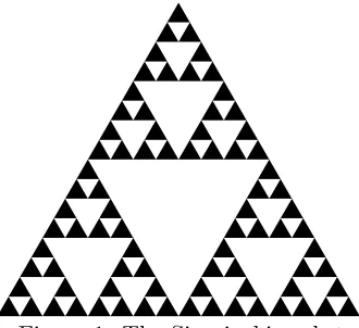
Figure 1: The Sierpinski gasket
2.2 P.c.f. self-similar sets and their Dirichlet forms
We call the self-similar set (K, S,{Fs}s∈S) a p.c.f fractal set if the post critical set P(L) is a finite set – p.c.f. here stands for ‘post critically finite’. This condition implies thatK is finitely ramified.
These sets were introduced by Kigami ([16]). In [16], [18], [20] it is shown that, provided a ‘non-degenerate harmonic structure’ exists, then a closed regular local Dirichlet form satisfying (2.1) exists, with the property that E(f, f) = 0, f ∈ F, implies that f is constant. (For work on the existence of non-degenerate harmonic structures see [25], [23].) In [16] the additional hypothesis of ‘regularity’ of the harmonic structure was imposed: in our context this means that the conductivitiesρi satisfy
ρi >1, ∀i∈S. (2.4)
We now summarise how the remainder of Assumption 2.3 is proved in this case. Because the resolvent operator is compact (see [18], [20]) andPtf =f if and only iff is constant, there is a spectral gap so that (2.3) holds.
Let Lµ be the self-adjoint operator on L2(K, µ) associated with the Dirichlet form (E,F), and let {λn}n be the eigenvalues of −Lµ and {ϕn}n be the normalized eigenfunctions. In [18], it is proved that ϕn is continuous and
kϕnk∞≤λκn n≥1,
whereκ depends only on the Dirichlet form andK. Thus, by Mercer’s theorem, pt(x, y) =
X
n
e−λntϕ
n(x)ϕn(y),
and the right hand side converges uniformly. This proves joint continuity of the transition density, and completes the verification of Assumption 2.3.
Let nµ(x) = #{λ:λis an eigenvalue of −L
µ ≤x.}. In [19], [18] it is proved that, ifdes(µ)>0 is the unique positive number satisfying
N
X
i=1
(µi/ρi)d
e
then
0<lim inf x→∞ n
µ(x)/xde
s(µ)/2 ≤lim sup
x→∞ n
µ(x)/xde
s(µ)/2 <∞.
In the case when (2.4) and (2.5) holds, let ν be the Bernoulli measure satisfying
νi =ρ−iσ ∀i∈S, (2.6)
where σ is the unique constant which satisfies PNi=1ρi−σ = 1. Then maxµdes(µ)/2 (where µ is taken to be a Bernoulli measure onK) is attained only atν, and the maximum value isσ/(σ+1). For this special case, (i.e. µ=ν) detailed estimates onpt(x, y) are obtained in [13]. We remark that if (2.4) holds then (2.2) is satisfied for any Bernoulli measure µ (with µi >0), and that des(µ)<2. In general, however, it is possible to have des(µ)>2.
2.3 Sierpinski carpets and their Dirichlet forms
LetH0 = [0,1]d, and let l∈N, l≥2 be fixed. Set Q={Π
d
i=1[(ki−1)/l, ki/l] : 1≤ki≤l, ki ∈
N (1≤i≤d)}, letl≤N ≤l
dand letF
i, 1≤i≤N be orientation preserving affine maps ofH0 onto some element of Q. (We assume that the sets Fi(H0) are distinct.) SetH1=∪i∈SFi(H0). Then, there exists a unique non-empty compact set K ⊂ H0 such that K = ∪i∈SFi(K) and (K, S,{Fs}s∈S) is a self-similar structure. K is called a Sierpinski carpet if the following hold: (SC1) (Symmetry)H1 is preserved by all the isometries of the unit cubeH0.
(SC2) (Connected) H1 is connected.
(SC3) (Non-diagonality) Let B be a cube in H0 which is the union of 2d distinct elements of
Q. Then if (H1∩B)o is non-empty, it is connected.
(SC4) (Borders included)H1 contains the line segment {x: 0≤x1 ≤1, x2 =· · ·=xd= 0}.
Here (see [5]) (SC1) and (SC2) are essential, while (SC3) and (SC4) are included for technical convenience. The main difference from p.c.f. self-similar sets is that Sierpinski carpets are infinitely ramified: the critical set C(L) in Definition 2.2 is infinite, and K cannot be disconnected by removing a finite number of points. In fact, for the classical Sierpinski carpet in R
d with l = 3 andN = 3d−1 we have V
0 = ∂[0,1]d. Write df = df(K) = logN/logl for the Hausdorff dimension of K. Note that the d-dimensional unit cube [0,1]d, d ≥ 2, can be included as an example of a Sierpinski carpet by takingN =ld.
We write ν for the Bernoulli measure with weights νi = 1/N: ν is a multiple of the Hausdorff measure onK. In [2], [21], [5], [14] a non-degenerate Dirichlet formE′ onL2(K, ν) is constructed on these spaces, with the property that E′ is invariant under local isometries of K – and in particularE′ is the same on each k-complex. The uniqueness ofE′ is an open problem – see [5]. IfE′ were unique then (2.1) would follow immediately. However, without requiring uniqueness,
in [21] (see also Remark 5.11 of [5] and [17]) a compactness argument is used to construct a Dirichlet form E with the same invariances as E′ and in addition satisfying (2.1) in the case when, for a constant ρK depending onK,
ρi =ρK, 1≤ ∀i≤N.
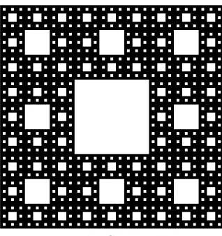
Figure 2: The Sierpinski carpet
dimension of K. When K = [0,1]d, Xb is just reflecting Brownian motion on [0,1]d, tK = l2 and ρK =l2−d. AsXb satisfies the same local isotropy condition as the processes studied in [2], [5], the techniques of those papers apply to Xb and lead to the same estimates for the Green’s function and transition density of the process.
Let µ be a Bernoulli measure satisfying (2.2). We now verify Assumption 2.3. For functions f, g, write f ≍g if there exists c1, c2 >0 such that c1g(x)≤f(x) ≤c2g(x) for all x. We have the following estimate of the 1-order Green’s kernel for the process X. The proof follows fromb the estimates and methods of [1], [4], [5].
Proposition 2.4 There exists a Green’s kernelbg1(x, y)which is continuous onK×K\ {x6=y}
(and on K×K when ds<2), and satisfies the following:
Ex[
Z ∞
0
e−tf(Xbt)dt] =
Z
Kb
g1(x, y)f(y)dν ∀f ∈ B(K),
b
g1(x, y) ≍
c2.2|x−y|dw−df if ds>2,
−c2.3log|x−y|+c2.4 if ds = 2,
c2.5 if ds<2.
We now wish to consider E on the space L2(K, µ), and to do this we use an argument due to Osada [24].
For an open setB ⊂K, define the capacity of B by
Cap(B) = inf{bE1(u, u) :u∈ F, u≥1 onB},
where forβ ≥0,Ebβ(u, u) =E(u, u) +βkuk2L2(K,ν). The capacity of any set F ⊂K is defined as the infimum of the capacity of open sets which containF. We say thatµcharges no set of zero capacity if the following holds:
µ(A) = 0 for all A∈ B(K) such that Cap(A) = 0.
Proof. If ds <2 then points have strictly positive capacity, and the result is immediate. We prove the result for ds > 2: the proof for ds = 2 is similar. It is well-known that for each compact setM ⊂K, Cap(M) ≥ µ(M)/c3 for each compact set M, thus for each Borel set, which completes the
proof.
As µ is a Radon measure which charges no set of zero capacity, it is a smooth measure in the sense of [9] (p. 80). Thus, it is a Revuz measure for some positive continuous additive functional A (see section 5.1 of [9]) and we can time change by the inverse of A – see section 6.2 of [9]. Dirichlet form on L2(K, µ). The next proposition shows that E =Ee, so that the Dirichet form is not affected by the time change.
Proposition 2.6 Assume (2.2). Then
IfK = [0,1]d this is just the classical Wiener test (see [15] or [22]); the result used here follows, using Proposition 2.4, by exactly the same arguments.
Using Kelvin’s principle (see Section 2.2 of [9]), we have for each compact set M ⊂K,
{Cap(M)}−1 = inf
Z
M×Mb
g1(x, y)m(dx)m(dy), (2.10)
where the infimum is taken over the positive Radon measures m with m(M) = 1. Now, take an arbitrary compact set M ⊂ Sn(x
K µ∗ <1 (due to assumption (2.2)) in the last inequality. Takingm(·) =µ(· ∩M)/µ(M) in (2.10), we have Cap(M)≥c5−1l−n(df−dw). As this holds for all
compact sets M ⊂ Sn(x0) with µ(M) ≥ µ(Sn(x0))/2, we have Cap(Sn(x0)) ≥ c−1
5 l−n(df−dw),
which proves (2.9).
We thus obtain a closed local regular Dirichlet form (E,Fe) onL2(K, µ) with the property (2.1): write X for the associated diffusion.
We next show that (2.3) holds. If ds < 2 then this is easy to verify directly. We omit the argument fords= 2: it follows by similar arguments to those fords>2.
For A ⊂ K write TA = inf{t ≥ 0 :Xt ∈ A}. Let x ∈ K−V∗, andσn = TDn(x)c. Let g(x, y)
be the (0th order) Green’s function for Xb killed on hitting Dn(x)c. From [5] we have that g(x, y) ≤c|x−y|dw−df. As the 0th-order Green’s function is not affected by the time change,
by a calculation similar to that in Lemma 2.5
Exσn = 6.14 goes through (with some modification) to prove that there exists β >0 such that
Then, by Ascoli-Arzel`a’s theorem, X has a compact resolvent. It is clear that Ptf =f if and only iff is constant. Thus there is a spectral gap, and (2.3) holds.
Finally, we prove the joint continuity of the transition density. As Pt is a self-adjoint compact operator onL2(K, µ), there existϕe
i that form a complete orthonormal system inL2(K, µ) with pt(x, y) =
∞ X
i=1
e−λitϕe
i(x)ϕei(y), forµ2-a.e. (x, y).
Further, the convergence is absolute and takes place in L∞(K×K) (see [5] Proposition 6.15). AsPtϕei=e−λiϕei a.e., we have Uλϕei= (λ+λi)−1ϕei a.e.. Defining ϕi= (λ+λi)Uλϕei, we have ϕi =ϕei a.e. and by (2.12), ϕi is continuous. On the other hand, by a routine argument from (2.3) plus hitting time estimates in Proposition 4.3 which will be proved later, we have
pt(x, x)≤c1t−γ1 ∀x∈K,0< t <1, (2.13) for some γ1 > 0 depending only on the Dirichlet form and µ (the detailed argument will be given for the killed process on DΛm(x) in Proposition 5.1). Note that this upper bound is not
sharp, but it is enough to deduce the continuity of pt(x, y). By this estimate, we see that
kPtk2→∞≤c1t−γ1/2. Thus,
kPtϕik∞=e−λitkϕik∞≤c1t−γ1/2 ∀i.
Takingt= 1/λi,kϕik∞≤c2λ−i γ1/2. Thus we can take a version of transition density as pt(x, y) =
X
n
e−λntϕ
n(x)ϕn(y),
and the convergence is uniform. This proves joint continuity of the density. We thus obtain a Dirichlet form on L2(K, µ) which satisfies Assumption 2.3.
3
Main Theorems
In the following, we identify Sn and the set of all n-complexes. For x, y ∈ K, we say Π =
{x, x1,· · ·, xl, y} is an m-walk of length |Π| =l+ 1 if x1,· · ·, xl ∈Sm, x∈Fx1(K), y ∈ Fxl(K)
and Fxi, Fxi+1 are adjacent m-complexes for 1 ≤i≤l−1. For simplicity, we will assume the following in the p.c.f. self-similar set case.
Assumption 3.1 Let L = (K, S,{Fs}s∈S) be a p.c.f. self-similar set. For each x, y∈ V0 with x6=y and for eachm≥0,
min{|Π|: Π is a m-walk from x to y} ≥2m.
We remark that if the self-similar structure L is changed to Ll = (K, Sl,{Fw}w∈Sl), then for
sufficiently largel,Llsatisfies Assumption 3.1. Forx∈K\V∗, letnr,j(x) be the shortest number of steps by a (Λr(x) +j)-walk from x to ∂DΛr(x). Further, for x∈K\V∗, define
pr(x) = min{k:x /∈DΛr(x)+k(∂DΛr(x))}.
Since ∩kDk(A) = A if A ⊂ K is closed, we have pr(x) < ∞ for x ∈ K \ V∗. Note that
Lemma 3.2 There exist c3.1 >0 such that the following holds for all r, j≥0 and x∈K\V∗.
e(j−pr(x))+/2 ≤2(j−pr(x))+ ≤n
r,j(x)≤c3.1e([logt ∗
]+1)j/2, (3.1)
where for x∈R, x+= max(x,0).
Proof. Using Assumption 3.1 in the p.c.f. case, and the fact that l≥2 in the carpet case, we have nr,j(x)≥2(j−pr(x))+. Since e <4 the first inequality is immediate.
Noting that if r ≥ nlogt∗ then Λ
r(x) > n for all x ∈ K −V∗, the third inequality can be
obtained by an easy modification of the proof of Lemma 3.3 in [13].
Now let µb be any Bernoulli measure on K so that µ(Vb 0) = 0, µ(Fb i(K)) = µbi for all i where
b
µi ≥0 satisfies Piµbi = 1. We emphasise that we continue to consider the density of X with respect to µ: the role of µb will be to select subsets of K with different limiting behaviour of pt(x, x).
As in [11], Lemma 6, we have
Proposition 3.3 There exists α >0 and g:K→ [0,∞) such that for µˆ-a.e. x∈K,
(rj)−αej/2 ≤nr,j(x)≤c3.1e([logt ∗
]+1)j/2 ∀r ≥0,∀j ≥g(x).
Proof. First note that ifx6∈Dk(V0) then anyj-walk fromxtoV0 requires at least 2j−k steps. Also, there existsθ <1 such thatµ(Db k(V0))≤c0θk fork≥1.
Since each Λn complex is a scaled copy ofK it follows that for 2≤k≤j,
b
µ({x:nr,j(x)≤2j−k})≤ c0θk. So, ifα0= log 2/log(1/ρ),
b
µ({x: 2−jnr,j(x)≤λ)≤c1λ1/α0 for 0< λ <1. So
b
µ({x: 2−jnr,j(x)≤λr−α0−1 for somer ≥0}) ≤
∞ X
r=0
b
µ(2−jnr,j(x)≤λr−α0−1)
≤ X
r
c1(λr−α0−1)1/α0 ≤c2λ1/α0.
Takingλ=j−α0−1 and applying Borel-Cantelli it follows that,µ-a.e.,b n
r,j(x)≥(rj)−α0−12j for all sufficiently largej. Puttingα=α0+ 1, the first inequality follows. The second inequality is
the same as in (3.1).
Theorem 3.4 There exists c3.2,· · ·, c3.8 >0 such that the following holds.
We note that in general n′ is not monotone increasing w.r.t. n. As we do not have a good comparison between pt(x, x) andpt/2(x, x), we need an extra logn′ in the time interval for the upper estimate. See the proof, which will be given in Section 5, for details.
Remark. For the p.c.f. fractals, we can also obtain the following estimate by the similar (but simpler) argument to the proof of Theorem 3.4.
There exist c3.9, c3.10, c3.11>0 such that for each x∈K and for each e−(n+1)≤t≤e−n,
Note that (3.2) always gives some estimate of the kernel for each fixedt whereas Theorem 3.4 does not (unlesstis small enough). On the other hand, whentis in the interval where Theorem 3.4 gives the estimate, it is much sharper than that of (3.2).
Concerning the lower bound for the p.c.f. fractals, (3.2) with c3.10 = 0, which is sharper than (3.2), is proved in Section 5 of [18]. For the p.c.f. fractals with a ‘regular harmonic structure’, sharper upper estimate of pt(x, x) is given in appendix of [12].
We cannot obtain (3.2) for the carpet cases asDΛ1n(x) could have a very ‘bad shape’ in general. When the sizes of two adjacent Λn-complexes inD1Λn(x) are very different, particles could escape
from DΛ1n(x) much faster than e−n.
Using Proposition 3.3, we have the following almost sure result.
Theorem 3.5 Let µb be a Bernoulli measure on K with weights µbi satisfying the hypotheses of
Proposition 3.3. There existc3.12, c3.13, c3.14 >0 and h:K→[0,1] such that
The proof is essentially the same as that of Theorem 3.4: we will remark on the necessary modifications in the last part of Section 5.
Corollary 3.6 The following holds for µˆ-a.e. x∈K: log(tx1. . . txn). Since, under µ,b xi are independent identically distributed random variables,
using the strong law of large numbersMk/k→Piµˆilogti for ˆµ−a.e. x∈K.
Finally, by Theorem 3.5, we have, µ-a.e.,b
lim
and using (3.5) and the law of large numbers completes the proof.
Remarks. 1) The formula for the ˆµ-a.e. spectral dimension (3.4) has the same form as that for the (stationary) homogeneous random Sierpinski gasket studied in [7]. However, in that case,
{µˆi}i corresponds to the frequency that each random pattern appears.
2) The condition (2.2) implies that 0 < ds(ˆµ) < ∞. Also, for the p.c.f. case with regular harmonic structure (2.4), we have ds(ˆµ)/2 < 1, as one expects. If µb is given by (2.6), then ds(ˆµ) =σ/(σ+ 1) and so is independent of ˆµ; this has already been proved in [13].
Note that while ds(µ)/2 ≥ des(µ)/2 (recall (2.5)), these two numbers are in general not equal. This lack of correspondence between the asymptotic growth of the eigenvalues and transition density emphasises the lack of uniformity in the behaviour ofpt(x, x).
3) Letσ(ˆµ) = (Piµˆilog(1/µi))/(Piµˆilogρi) whenPiµˆilogρi 6= 0. We can then write the introduction; some properties of this diffusion process were studied in [10]. For this case, log2(1/p)< σ(ˆµ)<log2(1/q) and by Proposition 4.7 in [10] (plus an easy Tauberian argument), the corresponding value for dyadic rational points is log2(1/p), the infimum of the interval. Using the continuity ofpt(x, x) and Corollary 3.6 one can show there exist points for which σ takes the maximum value log2(1/q).
5) If minilogρi/log(1/µi) 6= maxilogρi/log(1/µi), using Corollary 3.6 and the continuity of pt(x, y), one can prove by an elementary argument that there are (uncountably many) x such that limt→0logpt(x, x)/logtdoes not exist.
6) Theorem 1.1 now follows from remarks 3) and 5).
7) Using the methods of [6] and [18], together with the (worse) lower bound in (5.2), which will be used for the proof of Theorem 3.4, and a chaining argument we have
pt(x, y)>0 ∀t >0,∀x, y∈K.
4
Hitting time estimates
In this section, we will prove some hitting time estimates for the process which will be needed for the transition density estimates.
We first give some notation. For each x∈K and m≥0, we fix a m-complex which contains x and denote it asD∗
m(x). Note thatD∗m(x) =Dm(x) if x∈K\V∗. For x∈K and m≥0, let
D1m,∗(x) ={C :C is am-complex which intersects Dm∗(x).}
Let Λ∗r(x) be the length of the word of D∗Λr(x), and define D1Λ,∗
r(x)+l(x) to be the union of
(Λ∗
r(x) +l)-complexes which intersect DΛ∗r(x)+l(x). In the following, we will treat the case where
x0 ∈K, r, m≥0 satisfy
D1Λ,∗
r(x0)+m(x0)⊂D
∗
Λr(x0). (4.1)
Note that when (4.1) holds for the carpet case, all (Λ∗r(x0) +m)-complexes are same size, so thatD1Λ,∗
r(x0)+m(x0) is a cube (or square whend= 2).
We will consider the process onDΛ1,∗
r(x0)+m(x0) whose Dirichlet form is the same as that of{Xt} but whose measureµesatisfiesµ(Ke wv1···vn) =µw(µ∗)mµvm+1· · ·µvnfor each (Λ∗r(x0)+n)-complex Kwv1···vn ⊂Kw =D
∗
Λr(x0) and alln≥m. LetXetbe the process associated withE andL
2(K,
e
µ) killed on∂DΛ1,∗
r(x0)+m(x0). As before, we defineTA= inf{t≥0 :Xt∈A} forA⊂K, and write
TA(X) for the analogous hitting time fore X. We then have the following.e
Lemma 4.1 Let x0 ∈K, r, m≥0 satisfy (4.1).
1) There exist 0< c4.1 < c4.2 (independent ofx0, r, m) which satisfy the following, c4.1e−(r+mlogt
∗
)≤Ex0(T ∂D1Λ,∗
r(x0)+m(x0)
(X)),e Ex(T∂D1,∗
Λr(x0)+m(x0)
(X))e ≤c4.2e−(r+mlogt ∗
) ∀x∈D1,∗
Λr(x0)+m(x0). 2) There exist 0< c4.3, 0< c4.4 <1 (independent of x0, r, m) such that for all 0< t <1,
Px0(T ∂D1Λ,∗
r(x0)+m(x0)
(X)e ≤t)≤c4.3er+mlogt ∗
Proof. For the p.c.f. case, 1) can be proved by a simple modification of Lemma 3.5 in [13] (one can also prove it using Green’s density killed at ∂DΛ1,∗
r(x0)+m(x0)). For the carpet case, 1) is proved in the same way as Proposition 5.5 in [5].
2) now follows directly from 1), as in Lemma 3.6 of [13], or Lemma 3.16 of [1].
Note thatXetis a time change of Xt, so that the trajectory of{Xet} is the same as that of{Xt}, but thatXet moves faster thanXt. Therefore, we have
Px0(T ∂DΛ1,∗
r(x0)+m(x0)
(X)e ≤t)≥Px0(T ∂DΛ1,∗
r(x0)+m(x0)
(X)≤t).
Thus, we have from Lemma 4.1 2) that
Px0(T ∂D1Λ,∗
r(x)+m(x)
(X)≤t)≤c4.3er+mlogt ∗
t+c4.4, (4.2)
for each 0< t <1 and for each x0 ∈K, r, m≥0 which satisfies (4.1).
Now, for a processX onK and for n≥0, we define a sequence of hitting times as follows,
σ0n(X) = 0,
σ1n(X) = inf{t≥0 :Xt∈∂Dn1,∗(X0)}, σkn+1(X) = inf{t≥σnk(X) :Xt∈∂D1n,∗(Xσn
k)}, ∀k≥1,
Wkn = σnk(X)−σnk−1(X), ∀k≥1. We have the following estimate of the crossing time distribution.
Lemma 4.2 There exist c4.5, c4.6, c4.7>0 such that for all 0≤r, Px(T∂DΛ
r(x)≤c4.7t)≤c4.5exp{−c4.6nr,k(x)} 0<∀t <1,∀x∈K\V∗, (4.3) where k=k(r, z, t) = inf{j : nr,j(z)
er+jlogt∗ ≤t}.
Remark. Note that, from (3.1), k <∞ for each r, t, z.
Proof. As the result is clear whenk= 0, we consider the casek≥1. First, for eachn≥r≥0, set
ξr,n= sup{i:σin≤T∂DΛr(x)}.
By the structure of K, there exists c1>0 such that
c1nr,m≤ξr,Λr(x)+m ∀r, m≥0.
We also note that for each r, m ≥ 0 and k ≤ ξr,Λr(x)+m − 1, {W
Λr(x)+m
k }k behave like
{TD1,∗
Λr(x)+m(XσΛr(x)+m k−1
)}k so that
P(WΛr(x)+m
k ≤t|W
Λr(x)+m
j ,1≤j ≤k−1)≤c4.3er+mlogt ∗
holds for k≤ξr,Λr(x)+m−1 by (4.2) ((4.1) clearly holds in these cases). Using these facts, we
have for eachx∈K\V∗,
Px(T∂DΛ
r(x)≤c4.7t) ≤ P
x(
c1nr,kX−1(x)
i=1
WΛr(x)+k−1
i ≤c4.7t) (4.5)
≤ expc2(nr,k−1(x)er+(k−1) logt ∗
c4.7t) 1
2 −c3nr,k−1(x)
= exp(−c4nr,k−1(x))≤exp(−c5nr,k(x)),
where we use Lemma 1.1 of [2] and (4.4) in the second inequality, and in the last equality we choose c4.7 so that c41./72 < c3/c2 (c4 =c3−c2c14/.72). We thus obtain the result. Letβ ≡logt∗. For each c >0, set
kc =kc(n, x, t) = inf{j:
nn,j(x)
en+βj ≤ct/c4.7}. Then, by Lemma 4.2, we have for each 0< t <1 andx∈K\V∗,
Px(T∂DΛ
n(x)≤ct)≤c4.5exp{−c4.6nn,kc(x)}. (4.6)
We now have the following exponential decay of the distribution of hitting times.
Proposition 4.3 There existc4.8, γ > 0 such that for each x∈K\V∗,0< s <1 and for each
t≤e−n′ (n′=n+βpn(x)),
Px(T∂DΛn(x)≤st)≤c4.5exp(−c4.8s
−γ).
Proof. First, takea= min{1, β}/2>0 and take ¯m∈Zsuch that
e−(β−a)( ¯m+1) ≤s/c4.7< e−(β−a) ¯m. (4.7) Then, using (3.1),
nn,j en+βj ≥e
a(j−pn(x))−n−βj > s
c4.7
e−βpn(x)−n≥st/c4
.7 (4.8)
for all j≤m¯ +pn(x), t≤e−n−βpn(x) so that
ks(n, x, t)−1≥m¯ +pn(x). (4.9)
Thus,ks−1−pn(x)≥m. Now, from (3.1) and (4.9), we have¯
nn,ks(z)≥nn,ks−1(z)≥e
1
2(ks−1−pn(x))≥e12m¯
so that the right hand side of (4.6) is less thanc4.5exp(−c4.6e 1
2m¯). By (4.7),e 1
2m¯ ≥c1s−γwhere γ = (2(β−a))−1 and the proof is completed.
5
Transition density estimates
5.1 Lower bound
In this subsection, we will obtain the lower bound of the transition density.
Proof of Theorem 3.4 1). Set c3.3 = β and let s > 0 satisfy c4.5exp{−c4.8s−γ} ≤ 1/2. Then, by Proposition 4.3, we have
Px(T∂DΛ
n(x)≤st)≤1/2 ∀x∈K\V∗, ∀t≤e
−n′ .
Thus,Px(Xst∈DΛn(x))≥1/2. Now, using Cauchy-Schwarz,
(1/2)2 ≤Px(Xst∈DΛn(x))
2 = Z DΛn(x)
pst(x, y)µ(dy)
2
(5.1)
≤ µ(DΛn(x))
Z
DΛn(x)
pst(x, y)2µ(dy)
≤ µ(DΛn(x))p2st(x, x).
Hence we deduce that p2st(x, x)≥c1{µ(DΛn(x))}
−1.
In Lemma 5.1 of [13], one of the author proves similar results, but the proof is incomplete as it could be carried out only when k >0 where k, which appears in the proof, is defined similarly to ours. The proof can be completed following the argument of ours, using Proposition 4.3. By a similar argument, it is easy to prove the weaker estimate
c1{µ(D[1n/logt∗](x))}−1 ≤pt(x, x) ∀x∈K\V∗, ∀t≤c2e−n.
Since µ(D[1n/logt∗](x))≤c3(µ∗)c4n, we have
pt(x, x)≥c5t−γ2 ∀x∈K\V∗, 0<∀t <1, (5.2)
whereγ2=c4log(1/µ∗). This uniform (worse) lower estimate will be used later.
5.2 Upper bounds
In this subsection, we will obtain the upper bound of the transition density. For the purpose, we will first obtain the upper estimate of the kernel with Dirichlet boundary condition. For each x∈K and n≥0, let pDΛn(x)
t (x, y) be the transition density of the process killed at∂DΛn(x).
Proposition 5.1 There exists c5.1, c5.2 >0 such that for each x∈K, c5.1e−n≤t and m≤n, pDΛm(x)
t (x, x)≤c5.2{ min
w∈Λn Fw(K)⊂DΛ
m(x)
µw}−1.
Proof. Forw∈Λm write fw =f◦Fw and define
¯ fw =
Z
K
fw(x)µ(dx) =µ−w1
Z
Fw(K)
Note that for v ∈ F, ¯v = R vdµ = Pw∈Λmv¯wµw. In the following, we fix x, m and denote B =DΛm(x). Letu0 ∈ D(L) with u0 ≥0,Suppu0 ⊂B and ku0k1 = 1. Setut(x) = (P
Using the fact that kPtk1→∞≤ kPtk21→2,we deduce the result.
Proof of Theorem 3.4 2). The main step in the proof is to compare the transition densities of X killed at ∂DΛm(x) with those of the unkilled process. Write ¯X for X killed at ∂DΛm(x),
and letτ =T∂DΛ
m(x). First, by Proposition 4.3,
Px(τ ≤st)¯ ≤c4.5exp{−c4.8s−γ}, for ¯t≤e−m′
. Sett=st. We first assume¯ e−n′
≤t¯≤e−m′
for somem≤nand later determine the right value ofs(right interval fort) where the comparison of Dirichlet and Neumann boundaries holds. For k≥n defineBk=DΛk(x)⊂DΛn(x). Then
Z
Bk
Z
Bk
pt(z, y)µ(dz)µ(dy) =
Z
Bk
Pz(Xt∈Bk)µ(dz)
=
Z
Bk
Pz( ¯Xt∈Bk)µ(dz) +
Z
Bk
Pz(Xt∈Bk, τ < t)µ(dz)
The second term above equals
Z
Bk
Pz(Xt∈Bk, τ ≤t/2)µ(dz) +
Z
Bk
Pz(Xt∈Bk, t/2< τ < t)µ(dz) =J1+J2 (5.4)
Since the processX started with measure µis symmetric,
J2 = Pµ(X0 ∈Bk, Xt∈Bk, t/2< τ < t)
≤ Pµ(X0 ∈Bk, Xt∈Bk,∃s∈[t/2, t) :Xs∈∂DΛm(x))
= Pµ(Xt∈Bk, X0 ∈Bk,∃s∈(0, t/2] :Xs ∈∂DΛm(x))
= Pµ(X0 ∈Bk, Xt∈Bk, τ ≤t/2) =J1
Writea(t/2) = sup{ps(y, y) :y∈K, t/2≤s≤t}. We have
Pz(Xt∈Bk, τ ≤t/2) = Ez1(τ≤t/2)PXτ(Xt−τ ∈Bk) = Ez1(τ≤t/2)
Z
Bk
pt−τ(Xτ, y)µ(dy)
≤ Pz(τ ≤t/2)a(t/2)µ(Bk).
Combining these estimates, lettingk→ ∞, and using the continuity of pt(·,·), we deduce that
pt(x, x)≤ptDΛm(x)(x, x) + 2a(t/2)Px(τ ≤t/2). By (2.13) and (5.2), there existsa >0 such that
a(t/2)≤c1t−apt(z, z) ∀z∈K\V∗, 0<∀t <1.
pt(x, x)≤pDtΛm(x)(x, x) +c2t−apt(x, x) exp{−c3s−γ}. (5.5)
We thus obtain the result using Proposition 5.1.
Note for the proof of Theorem 3.5. First, it is enough to prove the following:
There exist C1,· · ·, C6 > 0 and k(x) < ∞ such that for ˆµ-a.e. x ∈ K and for each ¯n =
argument for the upper bound, we obtain Theorem 3.5. Note that by takingc3.12 large in (3.3), we can state the upper and lower bounds simultaneously.
Now, in order to apply the proof in this section for (5.6) and (5.7), the following modification is needed. First, takingc′ <1/2, we have by Proposition 3.3 that for ˆµ-a.e x∈K, there exists ¯
g(x)<∞ such that
r−αec′j ≤nr,j(x) ∀r≥0, ∀j ≥¯g(x). We will change the definition of kb so that
kb = inf{j ≥¯g(x) :
nr,j(x)
er+βj ≤bt/c4.7,
nr,j−1(x)
er+β(j−1) ≥bt/c4.7}. (5.8) Then (4.3) holds for thiskb(withbtinstead oft). Noting thatpr(x)/2 in Lemma 3.2 corresponds toαlogr in this case, it is not hard to modify Proposition 4.3 usingkb in (5.8). Then, the lower and upper bounds can be proved in the same way. The extra logn′term is taken intoC
2logn.
References
[1] M. T. Barlow, Diffusions on fractals, Lectures on Probability Theory and Statistics: Ecole d’Et´e de Probabilit´es de Saint-Flour XXV, Springer, 1998.
[2] M. T. Barlow and R. F. Bass, The construction of Brownian motion on the Sierpinski carpet, Ann. Inst. H. Poincar´e,25(1989), 225–257.
[3] M. T. Barlow and R. F. Bass, Local times for Brownian motion on the Sierpinski carpet, Probab. Theory Relat. Fields,85(1990), 91–104.
[4] M. T. Barlow and R. F. Bass, Transition densities for Brownian motion on the Sierpinski carpet,
Probab. Theory Relat. Fields,91 (1992), 307–330.
[5] M. T. Barlow and R. F. Bass, Brownian motion and harmonic analysis on Sierpinski carpets, Canad. J. Math.51 (1999), 673–744.
[6] M. T. Barlow, R. F. Bass and K. Burdzy, Positivity of Brownian transition densities, Elect. Comm. in Probab.,2(1997), 43–51.
[7] M. T. Barlow and B. M. Hambly, Transition density estimates for Brownian motion on scale irregular Sierpinski gasket, Ann. Inst. H. Poincar´e,33(1997), 531–557.
[8] M. T. Barlow and E. A. Perkins, Brownian motion on the Sierpinski gasket, Probab. Theory Relat. Fields,79(1988), 543–624.
[9] M. Fukushima, Y. Oshima and M. Takeda, Dirichlet forms and symmetric Markov processes, de Gruyter, Berlin, 1994.
[10] T. Fujita, Some asymptotic estimates of transition probability densities for generalized diffusion processes with self-similar speed measures, Publ. Res. Inst. Math. Sci., 26(1990), 819–840.
[11] B. M. Hambly and O. D. Jones, Asymptotically one-dimensional diffusion on the Sierpinski gasket and multi-type branching processes with varying environment, preprint 1998.
[12] B. M. Hambly, J. Kigami and T. Kumagai, Multifractal formalisms for the local spectral and walk dimensions, Maths. Proc. Cam. Phil. Soc., to appear.
[13] B. M. Hambly and T. Kumagai, Transition density estimates for diffusions on post critically finite self-similar fractals, Proc. London Math. Soc.,78(1999), 431–458.
[14] B. M. Hambly, T. Kumagai, S. Kusuoka and X. Y. Zhou, Transition density estimates for diffusion processes on homogeneous random Sierpinski carpets, J. Math. Soc. Japan,52(2000), 373–408.
[15] K. Itˆo and H. P. McKean, Jr.,Diffusion processes and thier sample paths (Second printing), Springer, Berlin, 1974.
[16] J. Kigami, Harmonic calculus on P.C.F. self-similar sets, Trans. Amer. Math. Soc., 335 (1993), 721–755.
[17] J. Kigami, Markov property of Kusuoka-Zhou’s Dirichlet forms on self-similar sets, J. Math. Sci. Univ. Tokyo,7(2000), 27–33.
[18] J. Kigami, Analysis on fractals, Cambridge Univ. Press, to appear.
[19] J. Kigami and M. L. Lapidus, Weyl’s spectral problem for the spectral distribution of Laplacians on P.C.F. self-similar fractals, Comm. Math. Phys.,158(1993), 93–125.
[21] S. Kusuoka and X. Y. Zhou, Dirichlet forms on fractals: Poincar´e constant and resistance, Probab. Theory Relat. Fields, 93(1992), 169–196.
[22] N. S. Landkof, Foundations of Modern Potential Theory, Springer, New York-Heidelberg, 1972.
[23] V. Metz, Renormalization contracts on nested frcatals,J. Reine Angew. Math.,480(1996), 161–175.
[24] H. Osada, A family of diffusion processes on Sierpinski carpets, Probab. Theory Relat. Fields, 119
(2001), 275–310.