FRACTAL ANALYSIS OF COLORS AND SHAPES FOR NATURAL AND
URBANSCAPES
J. H. Wang a, *, S. Ogawa b
a Nagasaki University, Graduate school of engineering, Bunkyo-machi, Nagasaki, 852-8521 Japan –[email protected]
b Nagasaki University, Graduate school of engineering, Bunkyo-machi, Nagasaki, 852-8521 Japan –[email protected]
KEY WORDS: amenity, box-counting, Brownian motion, natural landscape, urbanscape
ABSTRACT:
Fractal analysis has been applied in many fields since it was proposed by Mandelbrot in 1967. Fractal dimension is a basic parameter of fractal analysis. According to the difference of fractal dimensions for images, natural landscapes and urbanscapes could be differentiated, which is of great significance. In this paper, two methods were used for two types of landscape images to discuss the difference between natural landscapes and urbanscapes. Traditionally, a box-counting method was adopted to evaluate the shape of grayscale images. On the other way, for the spatial distributions of RGB values in images, the fractal Brownian motion (fBm) model was employed to calculate the fractal dimensions of colour images for two types of landscape images. From the results, the fractal dimensions of natural landscape images were lower than that of urbanscapes for both grayscale images and colour images with two types of methods. Moreover, the spatial distributions of RGB values in images were clearly related with the fractal dimensions. The results indicated that there was obvious difference (about 0.09) between the fractal dimensions for two kinds of landscapes. It was worthy to mention that when the correlation coefficient is 0 in the semivariogram, the fractal dimension is 2, which means that when the RGB values are completely random for their locations in the colour image, the fractal dimension becomes 3. Two kinds of fractal dimensions could evaluate the shape and the color distributions of landscapes and discriminate the natural landscapes from urbanscapes clearly.
1. Introduction
Landscape perception or preference as a valid indicator of the related policy which has been widely accepted by the development and environmental management department (Kaplan, 1988; Purcell et al., 1994; Lothian, 1999; Hagerhall, 2001; Brady, 2006). In natural phenomena there is often also a particular combination of complexity and coherence provided by patterns that repeat at different scales, such as a snowflake where a part of the snow flake is similar to the whole snowflake. According to the previous research, it is reasonable to assume for the existence of fractal nature in landscapes. A key advantage of the fractal dimension is that, within the range of the fractal dimension, it is a scale independent property(Ode, Hagerhall, & Sang, 2010). A considerable amount of research has been done to find the relationship between fractal dimension and landscape preference. Through calculating the fractal dimension of landscape silhouette outlines, Hagerhall, Purcell and Taylor(2004) found the relationship between preference and the fractal dimension D, which indicates that this particular geometry may be part of the basis for preference. In (Tveit, Ode, & Fry, 2006), fractal dimension was used as a potential indicator of naturalness that is one of the nine key visual concepts for analyzing the visual landscape character. In(Berling-wolff & Wu, 2004), the historical development of urban growth model was reviewed and the influence of fractal geometry on the urban growth model was acknowledged.
1.1 Fractal dimension
Fractal is defined as a shape has statistically self-similarity to
*Corresponding author. Tel. +81 958192611. E-mail address: [email protected]
some extent, which was proposed by Mandelbrot in 1967 (Mandelbrot, 1967). Fractal is a shape made of parts similar to the whole in some way. Fractal dimension is the basic parameter of fractal analysis. Researchers have proposed many methods to calculate the fractal dimension of different types of objects, including Hausdorff dimension, similarity dimension, compass dimension, box-counting dimension, information dimension, generalized dimension, correlation dimension and fractal Brownian motion (fBm) dimension. As defined in Hausdorff dimension. (Tricot, 1982) assumed the shape taken into account is bounded in Euclidean space, the fractal dimension is calculated by equation (1):
D = lim�→ log ��
more directly when there is a change. Thus, those can be reflected in the fractal dimension value of the RGB values distribution in the image.
1.2 Objectives
Generally, landscapes are divided into four terrestrial landscapes. Here landscapes are simply divided into two categories, natural landscapes and urbanscapes. With the rapid process of urbanization, there are more and more natural areas changing into urban areas. Urbanscapes are greatly different with natural landscapes in many aspects. The point now we interested in is that there are so many irregular shapes combination and conflicts in colors combination in city areas, which is hard to find in nature. Using fractal dimension D as a tool to detect the difference between natural landscapes and urbanscapes. In this paper, gray-scaled images and color images of landscapes were analyzed by different fractal dimension estimating methods to discuss the difference between natural landscapes and urbanscapes. For gray scale images, a box-counting method was used to calculate the fractal dimension. For color images, fractal Brownian motion (fBm) method was adopted to estimate the fractal dimension of the RGB value distribution in an image. In both of the two methods, a convenient, simple thought was implied to get the fractal dimension directly, without large amount of data works.
2. Method
A collection of natural and urbanized images were used to compare the fractal dimensions. In this paper, 8 natural images and 8 urbanized images were obtained to do analysis. For every single image, we estimate the fractal dimensions for shapes (FD) for shapes from the grayscale images and the fractal dimensions (FD) from color images. The FD for shapes were calculated using the well-known Box-counting method. The FD of color images were estimated employing the fractal Brownian model.
2.1 A simplified Box-counting method for grayscale images
The first box-counting method is described as equation (2), assumed the shape taken into account is a bounded set in Euroclidean space(Lovejoy, Schertzer, & Tsonis, 1987). The fractal dimension describes how many new pieces of the set are resolved as the resolution scale is decreased. Since a fractal is isotropic due to self-similarity, the fractal dimension could be estimated through any two directions. In practical, the differential equation is often used to estimate fractal dimension as shown in equation (3). To be easier, the fractal dimension is the slope of the fitting line which is obtained by fitting a set of points (log ��,log �)(Yong-qiang, An-sheng, Ìá, & Åäî, 2005). In this paper, the fitting line method was adopted. Two points definitely determine a straight line. Generally, it needs much computation work using the box-counting method(Liebovitch & Toth, 1989). To simplify the calculation, two extreme cases were taken into counted, that is, � � and � � . When r is equal to � �, that is, the side length of the photo, N is equal to �� � = . When r is equal to � � = , N is equal to �� �,
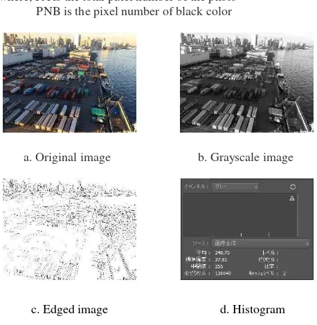
which could be obtained from the histogram. The fractal dimensions were obtained by equation (4). Using Laplacian operator, the edge-extraction image was obtained from grayscale images as shown in fig.1. �� � could be estimated by
is the least number of boxes to cover the shape by box with side length r.
where, PA is the total pixel number of the photo PNB is the pixel number of black color
a. Original image b. Grayscale image
c. Edged image d. Histogram
Figure 1. Process of calculation of FD of a grayscale image using the Box-counting method
2.2 Fractal Brownian motion model for color images
For a color image, the RGB values distribution is considered to be Brownian motion. Therefore, fractal Brownian motion model was adopted to estimate the fractal dimensions of the color images. The fractal dimension can be calculate according to the following equations (5) and (6) (Zou, 2012; Ogawa, 1995). H is the Hurst exponent (0< H<1). When H = 1/2, the distribution is a classical Brownian function(Pentland, 1984).
γ h = E[� − � ] = ℎ � (5)
H =log E[ − ]log ℎ 2 (6)
D = − H
where, γ h is the semivariogram of the distance between any two points on the photos
� and � is the RGB values of the two points A and B
h is the distance between the corresponding two points.
3. Results and discussion
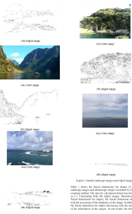
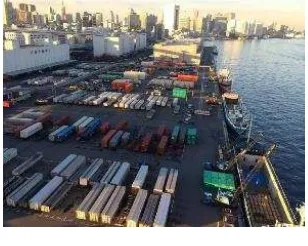
In this section, the fractal dimensions for shapes and fractal dimensions for colors were calculated. Then considering of the fractal dimension, analysis was done to compare natural landscapes with urbanscapes. The number of images used in the comparison is 8 natural landscape images and 8 urbanscape images, as shown in figure 3 and figure 4. Figure 3 and figure 4 both show the original colorful images and black and white edged images of natural and urbanized respectively. As shown in figure 3, the natural landscape images include grassland, flowers, mountains, lakes and seas. As shown in figure 4, the urbanscape images include Sculptures, parks, cities, tenement,
downtown area and Squares.
3.1 Fractal dimensions of shapes and comparison of natural landscape and urbanscape images.
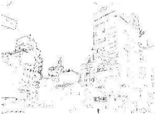
As shown in Figure 3 and 4, the right images is the edged image of the left images through Laplacian operator. Comparing the natural edged images with urbanized images, obviously we can found that the black point is more in urbanscape images than that in natural landscape images, which means that there is more sudden change in color in urbanized images.
(1a) Color image
(1b) Edged image
(2a) Color image
(2b) Edged image
(3a) Color image
(3b) Edged image
(4b) Edged image
(5a) Color image
(5b) Edged image
(6a) Color image
(6b) Edged image
(7a) Color image
(7b) Edged image
(8a) Color image
(8b) Edged image
Figure3. Natural landscape images and edged images.
for natural landscape images is in the range of 1.00 to 1.51.Among the 8 natural landscape images, as we can see, the smoothest one is No.8a image. As shown in the Table 1, the color FD value of No. 8 natural landscape images is the lowest, 1.00, which is in agreement with the visually impression. From Table 1 we can find that the No. 7natural landscape images is of largest FD value, 1.51, which means the image should be the coarsest one of all 8 natural landscape images. At the same time, from figure 3 we can find that the No.4a image indeed is coarser than other images.
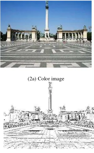
For urbanscape images the FD values is in the range of 1.27 to 1.53. Among them, No.2, No.4 and No.6 urbanized photos have larger FD values, that is, 1.53, 1.53 and 1.52 respectively. And from the Figure 4 we can visually find that the No.2a image, No.4a image and 6a image has larger color suddenly change than other images. At the same time, from the 8 urbanized images, it is not difficult to find that the No.2, No.4 and No.6 urbanized photos show more directly changing in color. In the same way, No. 1 urbanized photos shows the smallest FD values for shapes, 1.27. And as shown in Figure 4, the No.1 edged image shows the less directly change in color.
Table 1. Fractal dimensions for shapes of natural landscape images and urbanscape images.
From Table 1, we can obviously find that the fractal dimensions for shapes values of natural landscape images is much smaller than that of urbanscape images.
(1a) Color image
(1b) Edged image
(2a) Color image
(2b) Edged image
(3a) Color image
(3b) Edged image
(4a) Color image
FD 1 2 3 4 5 6 7 8
Natural 1.4
9 1.30 1.47 1.24 1.25 1.24 1.51 1.00 Urbanize
(4b) Edged image
(5a) Color image
(5b) Edged image
(6a) Color image
(6b) Edged image
(7a) Color image
3.2 Fractal dimensions of colors and comparison of natural landscape and urbanscape images
Table 2 shows the fractal dimensions for colors for natural landscape images and urbanscape images estimated by the fractal Brownian motion model. The specific calculation details has descripted in 2.2.Theoretically, for fractal dimensions for colors, as indicated in (Bisoi & Mishra, 2001), the smoother an image is, the closer its fractal dimension is to 2. On the other hand, the rougher an image is, the closer its fractal dimension is to 3. In our results, we can find the FD values is in the range of 2.61 to 2.75. Among 8 natural landscape images, the smoothest one is No.8a image. As shown in the Table 1, the color FD value of No. 8 natural photo is the lowest, 2.61, which is in agreement with the visually impression. From Table 1, the No. 4 natural photos is of largest FD value, 2.75, which means the image should be the coarsest one of all 8 natural images. Meanwhile, from Figure 3 we can find that the No.4a image indeed is coarser than other images.
(7b) Edged image
(8b) Edged image
Figure 4. Urbanscape images and edged images.
For urbanized images, the fractal dimension values were in the range of 2.75 to 2.81. Among them, the No.1 and No.3 urbanscape images have the lowest fractal dimension values, that is, 2.75. As shown in Figure 4, it seems like that the corresponding images show less directly change in color than other images. Moreover, from Table 2, the No.2, No.4 and No.7 urbanscape images is of larger fractal dimension values than other urbanscape images. From Figure 4, we can visually find that the corresponding images show more directly change in color than other images.
As shown in Table 2, the fractal dimensions for colors values of natural landscape images is also obviously smaller than that of urbanscape images.
Table 2. Fractal dimensions for colors of urbanscape images and natural landscape images.
3.3 comparison of fractal dimensions for shapes and fractal dimensions for colors
Comparing Table 1 with Table 2, we could find that for natural landscape and urbanscape images, the two kinds of fractal dimensions are of high agreement with each other. As for natural landscape images, the No.8 image has the smallest fractal dimensions for FD of shapes and FD of colors, 1.00 and 2.61 respectively; the No.6 images has the larger fractal dimensions than most of other images for FD of shapes and FD colors, 1.51 and 2.74 respectively. For urbanscape images, the No. 2 image has the largest fractal dimension, 2.81 and 1.51 for fractal dimension for colors and fractal dimension for shapes respectively; the No.1 image has smaller fractal dimension, 2.75 and 1.27 for FD colors and FD shapes respectively.
With the rapid process of urbanization, there are more and more natural areas changing into urban areas. Urbanscapes are greatly different with natural landscapes in many aspects. The point we interested in is that there are so many irregular shapes and directly colors combination in city areas, which is hard to find in nature. Table 3 shows the mean values of the two groups of images for fractal dimensions for colors and fractal dimensions for shapes. Compared the mean value of natural landscape images and urbanscape images, we can easily find that for both of the methods, the fractal dimensions of natural landscape
images is far smaller than that of urbanscape images. The fractal difference between them is 0.08 and 0.11 for fractal dimensions for colors and fractal dimensions for shapes respectively. The results verify well the difference in color and shapes between natural landscapes and urbanscapes.
Table 3. Comparison of the mean fractal dimensions of natural landscape images and urbanscape images.
Mean Natural Urbanized
CFD 2.70 2.78
SFD 1.31 1.42
CFD is the fractal dimensions for colors calculating from RGB values; SFD is the fractal dimensions for shapes calculating from the edged image.
3.4 Relationship between correlation coefficient and fractal dimensions for colors
Figure 5 shows the relationship between the fractal dimensions and the correlation coefficients for two kinds of landscape images. The correlation coefficient reflects the dependence of RGB distribution on spatial location. As shown in Figure 5, the fractal dimensions for colors decreases with the increase of independent with the spatial location, the fractal dimension for colors is 3.0.
Figure 5. Relationship between fractal dimensions and the correlation coefficients
4. Conclusions
In this paper, in the point of shapes and colors, the two kind of landscapes demonstrated different fractal dimensions. Fractal geometry is a great indicator for charactering the different landscapes. With the social development, more and more natural area are transferred to urban area. There is big difference between natural landscapes and urbanscapes. In this paper, two methods were used to estimate the fractal dimensions for color images and monochrome edged images. The results demonstrated significant difference in the mean fractal dimension values for two kinds of landscape images, 0.08 and 0.1 for fractal dimensions for shapes and fractal dimensions for colors respectively. The fractal dimensions for colors reflected the dependence of RGB values distribution on the spatial location. The fractal dimensions for colors decreased with the increase of the dependence of RGB values distribution on the spatial location. When the dependence was close to 0, the fractal dimension for colors was close to 3.0.
In this paper, we simply divided landscapes into two categories
FD 1 2 3 4 5 6 7 8
Natural 2.7
0 2.71 2.72 2.75 2.65 2.70 2.74 2.61 Urbanize
(natural and urbanized). In some cases, we could distinguish the natural landscapes from urbanized landscapes. In the future, we would analyze the four main terrestrial landscapes (agricultural, forested, arid and urban) and analyze the fractal dimensions difference among them.
5. Reference
Abe, T., & Ogawa, S., 1997. Fractal analysis for evaluating pavement performance. Art, Science and Practice (ASCE), Boston Mass.
Berling-wolff, S., & Wu, J., 2004. Modeling urban landscape dynamics : A review, (March 2003), pp. 119–129.
Bisoi, A. K., & Mishra, J., 2001. On calculation of fractal dimension of images. Pattern Recognition Letters, 22(6-7), pp. 631–637.
Brady, Emily., 2006. Aesthetics in practice: Valuing the natural world. Environmental Values, 15(3), pp. 277-291.
Hagerhall, C. M., Purcell, T., & Taylor, R., 2004. Fractal dimension of landscape silhouette outlines as a predictor of landscape preference. Journal of Environmental Psychology, 24(2), pp. 247–255.
Hagerhall, C. M., 2001. Consensus in landscape preference judgments. Journal of Environmental Psychology, 21(1), pp. 83-92.
Kaplan, Stephen., 1982. Where cognition and affect meet: A theoretical analysis of preference. EDRA: Environmental Design Research Association.
Li, J., Du, Q., & Sun, C., 2009. An improved box-counting method for image fractal dimension estimation. Pattern Recognition, 42(11), pp. 2460–2469.
Liebovitch, L. S., & Toth, T., 1989. A fast algorithm to determine fractal dimensions by box counting, Physics Letters A, 141(8), pp. 386–390.
Long, M., & Peng, F., 2013. A Box-Counting Method with Adaptable Box Height for Measuring the Fractal Feature of Images, pp. 208–213.
Lothian, Andrew., 1999. Landscape and the philosophy of aesthetics: is landscape quality inherent in the landscape or in the eye of the beholder?. Landscape and urban planning, 44(4), pp. 177-198.
Lovejoy, S., D. Schertzer, and A. A. Tsonis., 1987. Functional box-counting and multiple elliptical dimensions in rain. Science, 235 (4792), pp. 1036-1038
Mandelbrot, B., 1967. How long is the coast of britain? Statistical self-similarity and fractional dimension. Science (New York, N.Y.), 156(3775), pp. 636–8.
Ode, Å., Hagerhall, C. M., & Sang, N., 2010. Analysing Visual Landscape Complexity: Theory and Application. Landscape Research, 35(1), pp. 111–131.
Pentland, a P., 1984. Fractal-based description of natural scenes. IEEE Transactions on Pattern Analysis and Machine Intelligence, 6(6), pp. 661–74. Retrieved from
Purcell, Alan T., et al., 1994. Preference or preferences for landscape?. Journal of environmental psychology, 14(3). pp.195-209.
Tricot, Claude. , 1982. Two definitions of fractional dimension. Mathematical Proceedings of the Cambridge Philosophical Society, 91(01), pp. 57-54.
Tveit, M., Ode, Å., & Fry, G., 2006. Key concepts in a framework for analysing visual landscape character. Landscape Research, 31(3), pp. 229–255.
Yong-qiang, C., An-sheng, L. U., Ìá, Ö., & Åäî, Ð., 2005. Summary of image analysis method based on fractal, 26(7), pp. 1781–1784.