EVALUATING ERROR OF LIDAR DERIVED DEM INTERPOLATION FOR
VEGETATION AREA
Z. Ismail, M. F. Abdul Khanan*, F. Z. Omar, M. Z. Abdul Rahman, M. R. Mohd Salleh
Faculty of Geoinformation and Real Estate, Universiti Teknologi Malaysia, 81310 UTM Skudai, Johor, Malaysia - (zamriismail, mdzulkarnain, mdfaisal)@utm.my, [email protected] and [email protected]
KEY WORDS: LiDAR, DEM, Interpolation, GIS, Slope, RMSE
ABSTRACT:
Light Detection and Ranging or LiDAR data is a data source for deriving digital terrain model while Digital Elevation Model or DEM is usable within Geographical Information System or GIS. The aim of this study is to evaluate the accuracy of LiDAR derived DEM generated based on different interpolation methods and slope classes. Initially, the study area is divided into three slope classes: (a) slope class one (0° – 5°), (b) slope class two (6° – 10°) and (c) slope class three (11° – 15°). Secondly, each slope class is tested using three distinctive interpolation methods: (a) Kriging, (b) Inverse Distance Weighting (IDW) and (c) Spline. Next, accuracy assessment is done based on field survey tachymetry data. The finding reveals that the overall Root Mean Square Error or RMSE for Kriging provided the lowest value of 0.727 m for both 0.5 m and 1 m spatial resolutions of oil palm area, followed by Spline with values of 0.734 m for 0.5 m spatial resolution and 0.747 m for spatial resolution of 1 m. Concurrently, IDW provided the highest RMSE value of 0.784 m for both spatial resolutions of 0.5 and 1 m. For rubber area, Spline provided the lowest RMSE value of 0.746 m for 0.5 m spatial resolution and 0.760 m for 1 m spatial resolution. The highest value of RMSE for rubber area is IDW with the value of 1.061 m for both spatial resolutions. Finally, Kriging gave the RMSE value of 0.790m for both spatial resolutions.
1. INTRODUCTION
Light detection and ranging (LiDAR) can be a source of data for generating precise and directly georeferenced spatial information about the shape and surface characteristic of the earth. LiDAR is an established method for collecting very dense and accurate elevation data across landscapes, shallow-water areas and project sites. It is a type of an active remote sensing technique which is similar to radar but uses laser light pulses instead of radio waves for capturing 3D point clouds of the earth surface (Habib et. al., 2005).
In recent years, LiDAR has become the main data source for producing high resolution digital elevation model (DEM) or digital terrain model (DTM) (Raber et. al., 2007). Typically, a spatial resolution of 1 metre or higher can be obtained from various sources for example high density airborne LiDAR, high resolution aerial photogrammetry and high resolution satellite stereo images. On the other hand, LiDAR derived elevation has absolute accuracy of about 6 to 12 inches (15 to 30 centimetres) for older data and 4 to 8 inches (10 to 20 centimetres) for more recent data. Concurrently, relative accuracy (e.g., heights of roofs, hills, banks, and dunes) is even better.
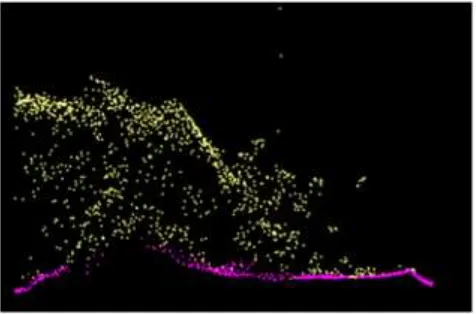
Nowadays, airborne LiDAR is a powerful tool to survey high resolution and high accuracy DEM for large areas (Wehr and Lohr, 1999). The output of an airborne LiDAR survey is a massive point clouds that needs to be interpolated in order to provide a continuous surface for final users (Kraus and Pfeifer, 2001). The choice of interpolator and the cell size play an important role for determining the quality of LiDAR-derived DEM (Bater and Coops, 2009). Figure 1.1 shows the result of point clouds that have been collected.
Figure 1. Example of point clouds captured by LiDAR. The yellow points show the treetop while the purple points indicate
ground points.
1.1 Digital Elevation Model
1.2 Slope
A slope is a change of elevation due to the change in horizontal position (Jones, 1998). Slope is regularly used to describe the steepness of the ground's surface where it can be measured as the rise (the increase in elevation in some unit of measure) over the run (the horizontal distance measured in the same unit as the rise) (Stump, 2001). GIS can analyze digital elevation data such as elevation points, contour lines and DEM and subsequently, derive both slope and aspect data sets from these elevation data. Later on, the slope and aspect data are used to describe landforms, to model surface runoff and to classify soils.
1.3 Interpolation
Interpolation according to Borrough et. al. (2001) is the procedure of predicting the value of attributes at unsampled site from measurements made at point locations within the same area or region. An interpolation made within a spatial context is known as spatial interpolation where it is the process of using the point with known values to estimate values at other points (Chang and Kang-tsung, 2006).
In general, there are two types of interpolation which are geostatistical and deterministic interpolations. Geostatistical interpolation is a method of surface creation by predicting the values between known values using the statistical approaches (Srivastava, 2006). On the other hand, deterministic interpolation creates surface based on measured points but does not take into account any spatial process occurs within (Anderson et al., 2005a). Several types of deterministic interpolations are Kriging, Inverse Distance Weighting (IDW), Spline and Natural Neighbours.
Kriging was originally developed to estimate the spatial concentrations of minerals for the mining industry and now is widely used in geography and spatial data analysis (Lee, 2004: Tang, 2005). Kriging assumes the distance or direction between the sample points that reflect a spatial correlation that can be used to explain variation in the surface. Kriging is essentially a weighted average technique but its weights depend not only on the distances between sample points and estimation locations but also on the mutual distances among sample points (Cressie, 1993; Desmet, 1997; Anderson et al., 2005a).
IDW assumes the closer a sample point is to the prediction location, the more it will influence the prediction value. According to Myers (1994), the assigned weight of IDW depends on the distance between the data location whereas the particular location estimation on the relative location between the sample data is not considered. IDW works well for dense and evenly distributed sample points (Child, 2004). Like Kriging, IDW uses a weighted average where the outside range of maximum and minimum sample point value is not estimated. Therefore, some important topographical features such as ridges and valley cannot be generated unless they have been sampled (Lee. 2004)
Finally, Spline interpolation uses a mathematical function that minimizes overall surface curvature. According to Johnston et al. (2001), Spline is an interpolator that fit a function to sampled points. Furthermore, this interpolator is able to estimate values that are below the minimum or above the maximum values within the sample data. This makes Spline
method effective for predicting ridges and valleys where usually sample date is not included (Child, 2004).
2. PROBLEM BACKGROUND
As reported by Su et al. 2006), IDW creates DEM with less overall error compared to other methods with an average error value of 0.116 m. On the other hand, Kriging and Spline methods provided the value of 0.133 m and 0.140 m each. He concluded by mentioning the accuracy of DEM varies with the changes in terrain and land cover type (Adams and Chandler, 2002; Hodgson and Bresnahan, 2004; Hodgson et al., 2005; Su and Bork, 2006). Similarly, research by Su and Bork (2006) stated that IDW is the most accurate interpolator with RMSE of 0.02 m lower than Spline and Kriging.
In their research, Liu et al. (2009) obtained RMSEs of 0.165 m by using Kriging, 0.174 m for IDW and 0.150 m using Local Polynomial (LP) on a flat terrain. However, on a complex terrain, the results were significantly different where IDW’s RMSE was 0.294 m, Kriging’s RMSE was 0.358 m and 0.25 m RMSE for Local Polynomial (LP) for site one which is in flat terrain. The fact that LP provided better results for the study was not significant it is a moderate quick interpolator compared to the IDW (Liu et al., 2009). Ideally again, IDW was seen as the best interpolation method.
However, research by Clark et al. (2004) provided a different result where Kriging gave an RMSE of 2.29 m compared to IDW which was 2.47 m. It is important to note that the research was carried out within a tropical rainforest surrounding where a mixture of old-growth terra firm, swamp, secondary and selectively logged forests, as well as agro-forestry plantations, developed areas with buildings and mowed grass, and abandoned pastures with large grasses, shrubs and remnant trees was the case.
There are many opinions regarding on which interpolation method produces the highest accuracy LiDAR DEM. It can be seen that IDW and Kriging are the main competitors when it comes to producing DEM when comparing RMSEs. To date, insufficient number of studies observed this LiDAR DEM interpolation accuracy issues for vegetated area.
According to Rasib et al. (2013), the combination of Kriging and Adaptive TIN (ATIN) algorithm for filtering method provides higher accuracy of DEM with RMSE values of 0.21 m for oil palm, 0.25 m for mixed forest and 0.32 m for mangrove. However, Razak et al. (2013) mentioned that IDW is still preferred as an interpolation technique due to its faster computational duration without adding artefacts to the DTM.
In addition to interpolation technique, slope can also affect the accuracy of DEM. Study by Salleh (2014) revealed that the highest RMSE is from a third class slope ranging from 11° to 15° with an RMSE value of 0.874 m compared to classes one and two slope with values of RMSE at 0.5964 m and 0.7232 m each. This study implemented Kriging interpolation technique.
LiDAR DEM accuracy are taken for granted within vegetated area. Therefore, this study is carried out to address this accuracy issue and to test the most suitable interpolation method especially for rubber estate and oil palm area.
2.1 Aim and Objectives
The aim of this study is to identify the accuracy of LiDAR DEM for vegetated area using different interpolation methods and slope classification. In order to achieve the aim of the study, three objectives have been developed:
1. To review selected interpolation methods
2. To generate DEM according to different interpolation methods and at different slope classes
3. To evaluate the accuracy of DEM using specific criteria
3. METHODOLOGY
3.1 Descriptions of Data and Study Area
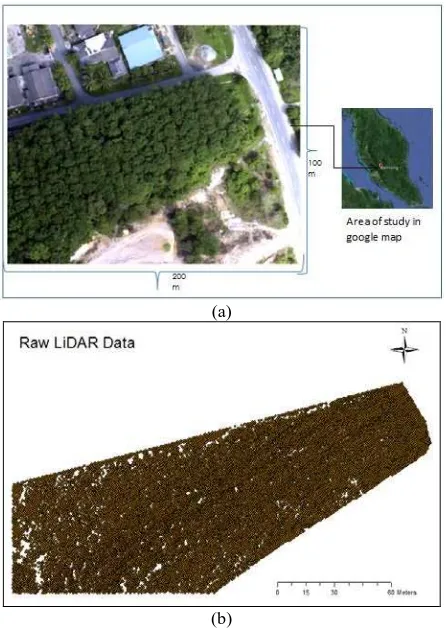
Figure 2 (a) and 3 (b) show the study area for this study while Figure 2 (b) and 3 (b) show the raw LiDAR data. The study area located at Simpang Pelangai, in district of Bentong, Pahang. The areas covered in this study are oil palm (150 m x 100 m) and rubber (200 m x 100 m).
The LiDAR data were collected on January 2009 using a REIGL laser scanner mounted on a British Nomad aircraft. The data were delivered in the classified LAS format of three-dimensional point cloud. The average LiDAR data sampling density across the area is about 2.2 points per m2.
(a)
(b)
Figure 2. (a) Map of study area Simpang Pelangai, Bentong, Pahang for rubber area, and (b) raw LiDAR data
(a)
(b)
Figure 3. (a) Map of study area Simpang Pelangai, Bentong, Pahang for oil palm area, and (b) raw LiDAR data
Field survey data is observed using tachymetry technique using total station and optical-levelling. In total, there are 132 points and 126 points of field survey data collected in rubber and oil palm areas, respectively. These points are collected based on the local Pahang State Cassini coordinate system, later on transformed to the old Malaysia Rectified Skew Orthomorphic (MRSO) using a general conversion method in GIS software.
3.2 Research Methodology
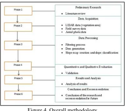
Figure 4. Overall methodology
3.2.1 Ground Filtering of LiDAR data
The purpose of ground filtering is to separate ground and non-ground data. The entire non-non-ground points that include vegetation and building are removed. Filtering of ground point is performed using Adaptive TIN (ATIN) approach that is embedded within TerraScan software. Suitable values of parameters are necessary in order to obtain a better filter. The parameters are:
1. Maximum building size 2. Iteration angle 3. Terrain angle 4. Iteration distance
Table 1 shows the values for each parameter that were used in TerraScan software for filtering process.
Parameters Value
Maximum building size 20 metre Maximum terrain angle 20 degree Maximum iteration angle 3.5 degree Iteration distance 1 metre Reduce iteration 1.2 metre Table 1. Value for Each Parameter in TerraScan
The maximum building size defines the area that will have at least one hit on the ground. On the other hand, the maximum terrain angle is the maximum of steepest allowed slope. The maximum iteration angle is the maximum angle between points while the iteration distance makes sure that the iteration does not produce big jump upward when triangles are large. Finally the reduce iteration parameter helps to avoid adding unnecessary point density to the group model. The optimum parameters are selected by examining topographic changes in the study area and comparing unfiltered and filtered results as an output iteratively. For the rubber area, the raw LiDAR points are 32447 and become 2670 after filtered. Meanwhile, for the oil palm area, the raw LiDAR points are 30498 and became 2867 after filtered. Table 2 summarizes the results of raw and filtered data for both oil palm and rubber areas.
Area Raw points Filtered points
Rubber 32447 2670
Oil palm 30498 2867
Table 2. Summarization of raw and filtered points for oil palm and rubber areas
3.2.2 DEM Generation Using Different Interpolation Methods:
Different interpolation methods result in different accuracy of the resultant DEM. Two types of DEM are produced from this study based on different data sources. The first DEM is from filtered LiDAR data while the second one is from tachymetry data. The DEM generated from tachymetry data is used as a reference and to produce slope maps. In this study, several interpolation techniques based on geostatistical approaches are selected due to their familiarity with DEM. The interpolation techniques are Kriging, IDW and Spline. The DEM generated from the filtered LiDAR data is interpolated using 0.5 m and 1 m of spatial resolution. Basically, the determination of spatial resolution is based on density and space between points (Meng et al., 2010). This should be done according to the density of ground points after the filtering and the need of the target application. For example 1 m spatial resolution can be generated with 2 point per m2 ground points. Certainly for 0.5 m DTM, a higher density of ground points after filteration is needed.
Interpolation is carried out using Geostatistical Analyst Tools in ArcGIS 10.2 software. Initially, the conversion of the LiDAR data from ASCII format to feature class format are carried out that precedes the interpolation step.
3.2.3 Slope Classification and Slope Map:
The quality of slope also contributes to the accuracy of the produced DEM. Here, the slope was generated from the DEM of field survey data. Slope tools in ArcGIS were used to produce the slope. Then the slopes are classified manually by using select by attribute of the raster value produced by slope. Table 3 shows the classification of the slopes
Slope class Slope range (degree)
1 0 – 5
6 – 10 11 – 15 2
3
Table 3. Slope classification based on slope range
3.2.4 Accuracy Assessment of LiDAR Derived DEM:
Corresponding bare-earth elevations are extracted from each LiDAR derived DEM at each point to assess the effect of slope category and filtering method on DEM error. Several methods are proposed for the assessment of the quality of the DEM. Mean signed error (MSE) and root mean square error (RMSE) are two commonly accepted statistical measurements used to assess DEM accuracy. Several studies used RMSE values based on high-grade in situ surveyed elevations to determine the accuracy of DEM across varying land cover and topography (Hodgson and Bresnahan, 2004; Bater and Coops, 2009; Spaete et al., 2011). Hodgson and Bresnahan (2004) and Su and Bork (2006) embedded MSE in to identify the tendency for under or over estimation of elevations relative to specific treatment classes.
n 2
( ZDEM ZREF) i 1
RMSE
n
∑ −
=
= (1)
where ZDEM = elevation derived from the LiDAR points ZREF = elevation derived from tachymetry data n = total number of points
Geostatistical Analyst Tool was again used to compare the results of LiDAR derived DEM against the tachymetry data derived DEM. The prediction of elevation from LiDAR derived DEM is automatically generated in an attribute table with the resultant error. Figure 5 shows the error generated from LiDAR derived DEM. The calculation of RMSEs was later on done using Microsoft Excel software.
Figure 5. Error generated from LiDAR derived DEM. Elevation values are from the reference data while predicted values are
elevation from LiDAR derived DEM
4. RESULTS AND DISCUSSION
4.1 Generated DEM
Two types of DEM are produced from this study. They are DEM from tachymetry data and DEM from LiDAR points.
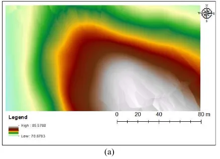
4.1.1 DEM from Tachymetry Data: There are two sets of tachymetry data; oil palm and rubber. Both tachymetry data are interpolated using Kriging technique for slope map creation. Figure 6 shows the results of DEM created from both tachymetry data.
(a)
(b)
Figure 6. DEM generated from tachymetry data for: (a) rubber area, (b) oil palm area
Kriging technique is solely used for generating the DEM from tachymetry data due to its performance. This technique performs better when compared to the other interpolation techniques in most contexts (Arun, 2013). In addition, Kriging produced better estimations of elevation especially when sampling points become sparse (Lloyd and Atkinson, 2006).
4.1.2 LiDAR Derived DEM for the Rubber Area:
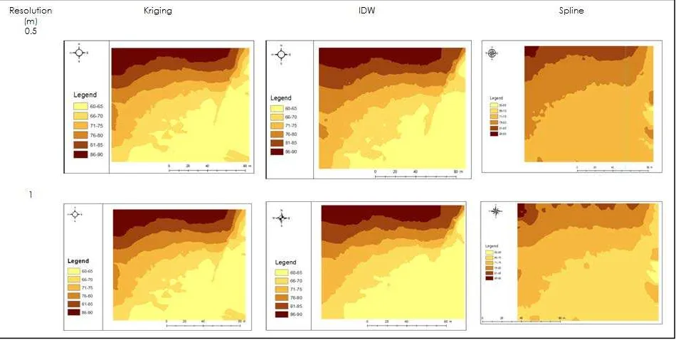
Two spatial resolutions of 0.5 m and 1.0 m are tested using three interpolation techniques. Figure 7 shows the LiDAR derived DEM using three interpolation methods with spatial resolution of 0.5 m and 1 m for the rubber area.
Based on Figure 7, Kriging produced the smoothest surface compared to IDW and Spline techniques. Spline technique generates corrugated surface compared to IDW for both 0.5 m and 1 m of spatial resolutions. It is also obvious that the highest elevation is from Spline interpolator at 85.5262 m.
4.1.3 LiDAR Derived DEM for the Oil Palm Area:
Similarly, two spatial resolutions of 0.5 m and 1 m are used for generating DEM of the oil palm area On top of that, three interpolation techniques are again tested which are Kriging, IDW and Spline. Figure 8 depicts the results of LiDAR derived DEM for 0.5 m and 1.0 m spatial resolutions for oil palm area.
4.2 Slope Map of Tachymetry Data
Slope is also one of the factors that need to be considered. Slope map was created from the DEM of tachymetry. Figure 9 show the slope map of both oil palm and rubber area. Based on Figure 8, Spline interpolator provides DEM with more corrugated surface, coarser tones and coarser texture compared to the DEM from IDW and Kriging interpolators. For Kriging and IDW techniques, there is no difference in the DEMs produced for both spatial resolutions. However, for Spline, it can be seen that there is a slight difference for both
4.3 Accuracy Assessments
spatial resolutions.
Figure 7. DEM generated for spatial resolutions of 0.5 m and 1 m for rubber area using Kriging, IDW and Spline interpolator
(a)
(b)
Figure 9. Slope map generated from DEM of (a) rubber area, (b) oil palm area
4.3.1 Overall Error Based on Interpolation Methods:
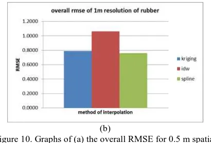
Table 4 shows the values of RMSE for the DEM of the rubber area and Figure 10 highlights the graph of the overall RMSE for the similar area. Similarly, Table 5 shows the values of RMSE for the DEM of the oil palm area and Figure 11 highlights the graph of the overall RMSE for the similar area.
Resolution (m) Methods RMSE (m)
0.5 Kriging 0.7895
IDW 1.06139
Spine 0.7463
1 Kriging 0.7895
IDW 1.0614
Spline 0.76
Table 4. The overall RMSE values of the rubber area
(a)
(b)
Figure 10. Graphs of (a) the overall RMSE for 0.5 m spatial resolution and, (b) the overall RMSE for 1.0 m spatial
resolution for the rubber area
Resolution (m) Methods RMSE (m)
0.5 Kriging 0.7266
IDW 0.7843
Spine 0.7338
1 Kriging 0.72662
IDW 0.7843
Spline 0.7475
Table 5. The overall RMSE values of the oil palm area
(a)
(b)
Figure 11. Graphs of (a) the overall RMSE for 0.5 m spatial resolution and, (b) the overall RMSE for 1.0 m spatial
4.3.2 Error Based on Slope Class:
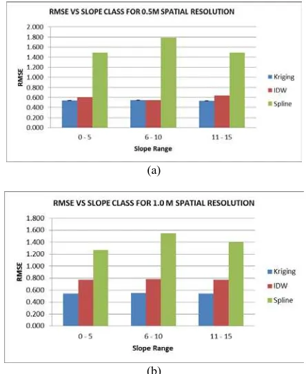
The discussion of this section is for two distinctive spatial resolutions, 0.5 m and 1.0 m, both for oil palm and rubber areas. For both spatial resolutions, three interpolations are tested. The calculation of RMSE based on slope class was done manually by classifying the raster value according to the slope range as mentioned in Table 3.
4.3.2.1 Rubber Area: The result of RMSE based on three interpolation methods and slope classes for both spatial resolutions of 0.5 m and 1 m is shown in Table 6 and Figure 12.
Spatial Resolution (m)
Slope Range (°)
Slope Class
Method RMSE
0.5 1 - 5 1 Kriging 0.626
IDW 0.68 Spline 0.801 6 - 10 2 Kriging 0.787 IDW 1.118 Spline 0.729 11- 15 3 Kriging 0.853 IDW 0.911 Spline 0.8
1 1 - 5 1 Kriging 0.655
IDW 0.694 Spline 0.76 6 - 10 2 Kriging 0.75 IDW 1.026 Spline 0.741 11- 15 3 Kriging 0.961 IDW 1.268 Spline 0.83 Table 6. RMSE according to slope classes of 0.5 m and 1m
spatial resolutions for rubber area
(a)
(b)
Figure 12. Graphs of RMSE versus slope class for spatial resolution of 0.5m and 1.0 m for rubber area
4.3.2.2 Oil Palm Area: Table 7 and Figure 13 show the result of RMSE based on three interpolation methods and slope classes for both, 0.5 m and 1.0 m spatial resolutions.
Spatial Resolution (m)
Slope Range (°)
Slope Class
Method RMSE
0.5 1 - 5 1 Kriging 0.542
IDW 0.544 Spline 0.533 6 -10 2 Kriging 0.603 IDW 0.545 Spline 0.64 11- 15 3 Kriging 1.49 IDW 1.785 Spline 1.491
1 1 - 5 1 Kriging 0.546
IDW 0.548 Spline 0.542 6 -10 2 Kriging 0.772 IDW 0.787 Spline 0.769 11- 15 3 Kriging 1.266 IDW 1.554 Spline 1.402 Table 7. RMSE according to slope classes of 0.5 m and 1m
spatial resolutions for oil palm area
From previous tables and figures within this section, it can be seen that different spatial interpolation methods have distinctive effects to the LiDAR derived DEM output. In general, Kriging provides the highest accuracy when compared against IDW and Spline for both study areas. This is due to the ability of Kriging where it examines specific sample points to obtain a value for spatial autocorrelation that
(a)
(b)
is only used for estimating surrounding points rather than assigning a universal distance power value. Furthermore, Kriging allows for interpolated cells to exceed the boundaries of the sample range (David et al. ,2005).
In relation to slope class, it can be seen that slope class 11° - 15° give the lowest accuracy for both study areas and spatial resolutions. Accuracy assessment using spatial resolution indicates that, the lower the spatial resolution is, the higher accuracy can be achieved. This is similar with Spaete et al., (2010) where he indicates that RMSE for slope greater than 10 degree provides greater values compared to slope class less than ten degree.
5. CONCLUSION
Both, interpolation method and slope class have effects towards the accuracy of DEM derived from LiDAR. From this study, IDW method give the lowest accuracy to the DEM while Kriging method can provide high accuracy of DEM produced in both areas. However, spline interpolator give the lowest value of RMSE for rubber area. For class slope, class slope 1 which are in the range of 1 – 5 degree give lowest accuracy for both area using different methods.
REFERENCES
Aguilar, F. J. and Mills, J. 2008. “Accuracy assessment of LiDAR‐derived digital elevation models.” The Photogrammetric Record 23(122): 148-169.
Anderson, ES, JA Thompson, and RE Austin. 2005. "LiDAR Density and Linear Interpolator Effects on Elevation Estimates." International Journal of Remote Sensing 26 (18): 3889-3900.
Arun, P. V. 2013. “A comparative analysis of different DEM interpolation methods.” The Egyptian Journal of Remote Sensing and Space Science 16(2): 133-139.
Burrough, P.A., and M.R. A. 1998. Principles of Geographical Information Systems. Oxford: Oxford University Press.
Chang, K. 2012. Introduction to Geographic Information Systems with Data Set Cd-Rom: McGraw-Hill Education.
Chang, K.. 2014. Introduction to Geographic Information Systems: McGraw-Hill Education.
Chang, Y, A Habib, D Lee, and J Yom. 2008. "Automatic Classification of LiDAR Data into Ground and Non-Ground Points." International archives of Photogrammetry and Remote Sensing 37: 463-468.
Child, C. 2004. Interpolating Surfaces in Arcgis Spatial Analyst. ArcUser, July - September 2004, 32-35.
Clark, Matthew L, David B Clark, and Dar A Roberts. 2004. "Small-Footprint LiDAR Estimation of Sub-Canopy Elevation and Tree Height in a Tropical Rain Forest Landscape." Remote Sensing of Environment 91 (1): 68-89.
Clark, Matthew L, David B Clark, and Dar A Roberts. 2004. "Small-Footprint LiDAR Estimation of Sub-Canopy Elevation
and Tree Height in a Tropical Rain Forest Landscape." Remote Sensing of Environment 91 (1): 68-89.
Habib, Ayman, Mwafag Ghanma, Michel Morgan, and Rami Al-Ruzouq. 2005. "Photogrammetric and LiDAR Data Registration Using Linear Features." Photogrammetric Engineering & Remote Sensing 71 (6): 699-707.
Hodgson, Michael E, and Patrick Bresnahan. 2004. "Accuracy of Airborne LiDAR-Derived Elevation." Photogrammetric Engineering & Remote Sensing 70 (3): 331-339.
Hodgson, Michael E, John Jensen, George Raber, Jason Tullis, Bruce A Davis, Gary Thompson, and Karen Schuckman. 2005. "An Evaluation of LiDAR-Derived Elevation and Terrain Slope in Leaf-Off Conditions." Photogrammetric Engineering & Remote Sensing 71 (7): 817-823.
Jamaludin, Suhaimi, and Ahmad Nadzri Hussein. 2006. "Landslide Hazard and Risk Assessment: The Malaysian Experience." Notes.
Jones, Kevin H. 1998. "A Comparison of Algorithms Used to Compute Hill Slope as a Property of the Dem." Computers & Geosciences 24 (4): 315-323.
Kraus, Karl, and Norbert Pfeifer. 2001. "Advanced Dtm Generation from LiDAR Data." International Archives Of Photogrammetry Remote Sensing And Spatial Information Sciences 34 (3/W4): 23-30.
Lee, Hyun Seung. 2004. "A Hybrid Model for Dtm Generation from LiDAR Signatures." Mississippi State University.
Li, Zhilin, Christopher Zhu, and Chris Gold. 2004. Digital Terrain Modeling: Principles and Methodology: CRC press.
Li, Zhilin, Christopher Zhu, and Chris Gold. 2004. Digital Terrain Modeling: Principles and Methodology: CRC press.
Liu, Xiaoye. 2008. "Airborne LiDAR for Dem Generation: Some Critical Issues." Progress in Physical Geography 32 (1): 31-49.
Lloyd, C. D. and Atkinson, P. M. 2006. “Deriving ground surface digital elevation models from LiDAR data with geostatistics.” International Journal of Geographical Information Science 20(5): 535-563.
Meng, Xuelian, Nate Currit, and Kaiguang Zhao. 2010. "Ground Filtering Algorithms for Airborne LiDAR Data: A Review of Critical Issues." Remote Sensing 2 (3): 833-860.
Myers, Donald E. 1994. "Spatial Interpolation: An Overview." Geoderma 62 (1-3): 17-28.
Raber, George T, John R Jensen, Michael E Hodgson, Jason A Tullis, Bruce A Davis, and Judith Berglund. 2007. "Impact of LiDAR Nominal Post-Spacing on Dem Accuracy and Flood Zone Delineation." Photogrammetric engineering & remote sensing 73 (7): 793-804.
Symposium-IGARSS: IEEE.
Razak, Khamarrul Azahari, Michele Santangelo, Cees J Van Westen, Menno W Straatsma, and Steven M de Jong. 2013. "Generating an Optimal Dtm from Airborne Laser Scanning Data for Landslide Mapping in a Tropical Forest Environment." Geomorphology 190: 112-125.
Renslow, Mike, Paul Greenfield, and Tony Guay. 2000. "Evaluation of Multi-Return LiDAR for Forestry Applications." US Department of Agriculture Forest Service-Engineering, Remote Sensing Applications. http://www. ndep. gov/USDAFS/LiDAR. pdf [Consulta: 12 de marzo de 2009].
Salleh, M. R. M. 2014. "Accuracy Assessment of LiDAR Derived Digital Elevation Model (Dem) with Different Slope and Different Canopy Density." Universiti Teknologi Malaysia.
Sithole, George, and George Vosselman. 2001. "Filtering of Laser Altimetry Data Using a Slope Adaptive Filter." International Archives of Photogrammetry Remote Sensing and Spatial Information Sciences 34 (3/W4): 203-210.
Spaete, Lucas P, Nancy F Glenn, Dewayne R Derryberry, Temuulen T Sankey, Jessica J Mitchell, and Stuart P Hardegree. 2011. "Vegetation and Slope Effects on Accuracy of a LiDAR-Derived Dem in the Sagebrush Steppe." Remote Sensing Letters 2 (4): 317-326.
Stump, Sheryl L. 2001. "High School Precalculus Students' Understanding of Slope as Measure." School Science and Mathematics 101 (2): 81-89.
Su, Jason, and Edward Bork. 2006. "Influence of Vegetation, Slope, and LiDAR Sampling Angle on Dem Accuracy." Photogrammetric Engineering & Remote Sensing 72 (11): 1265-1274.
Su, Jason, and Edward Bork. 2006. "Influence of Vegetation, Slope, and LiDAR Sampling Angle on Dem Accuracy." Photogrammetric Engineering & Remote Sensing 72 (11): 1265-1274.
Svobodová, JANA, and PAVEL Tuček. 2009. "Creation of Dem by Kriging Method and Evaluation of the Results." Geomorphologia Slovaca et Bohémica 9 (1): 53-60.
Tang, Tao. 2005. "Spatial Statistic Interpolation of Morphological Factors for Terrain Development." GIScience & Remote Sensing 42 (2): 131-143.
Wechsler, Suzanne P. 2003. "Perceptions of Digital Elevation Model Uncertainty by Dem Users." URISA-WASHINGTON DC- 15 (2): 57-64.
Wechsler, Suzanne P. 2011. Development of a LiDAR Derived Digital Elevation Model (Dem) as Input to a Metrans Geographic Information System (Gis).
Wehr, Aloysius, and Uwe Lohr. 1999. "Airborne Laser Scanning—an Introduction and Overview." ISPRS Journal of photogrammetry and remote sensing 54 (2): 68-82.