ACCURACY ANALYSIS OF HRSI-BASED GEOPOSITIONING USING LEAST
SQUARES COLLOCATION
Yunzhong Shen1,2, Chuang Li1,2, Gang Qiao1,2, and Shijie Liu1,2
1. Dept. of Surveying and Geo-informatics Engineering, Tongji University, Shanghai, PR,
China
2. Center for Spatial Information Science and Sustainable Development, Shanghai, PR, China
yzshen@tongji.edu.cn
KEY WORDS: Geopositioning, QuickBird Imagery, Rational Function Model, Stochastic Model, Variance Components
Estimation, Least Squares Collocation
ABSTRACT:
Rational function model with bias compensation has been widely used in geopositioning of High Resolution Satellite Imagery (HRSI). We studied the geopositioning issue using a pair of QuickBird imagery in the Shanghai urban area with 126 Control Points (CPs) measured by GPS RTK. We proposed in this paper a stochastic model of HRSI geopositioning in which we modeled the random observed error and signal parts, then the Least Squares Collocation (LSC) is suggested to process the geopositioning with such kind of stochastic model. In order to correctly determine the variance components of the observed random error and signal parts, the variance components estimation of MINQUE is applied to compute the variance components for the LSC approach. And the cofactor matrix of signals is computed according to a prior given function. Then the same pair of QuickBird imagery is processed by using LSC approach with the stochastic model of this paper. In the experiments parts of the CPs are used as Ground Control Points (GCPs) to compute the bias-corrected parameters and parts of them are used as check points to calculate the root mean square errors for different schemes. Experimental results show that the proposed LSC approach for affine transformation model could improve geopositioning accuracy significantly, about 15 cm numerically (15% on average), even better than second-order bias-corrected model with the same GCPs.
1. INTRODUCTION
Since the rigorous physical models of geopositioning are complicated and depended on sensor types, whose parameters are confidential by some commercial satellite imagery vendors, the rational function model (RFM) has drawn great interests and been extensively investigated in the last decades, and it has been proved to be an ideal replacement of rigorous physical models (Madani, 1999; Dowman and Dolloff, 2000) and adopted by OGC (Open Geospatial Consortium) as one of the standard image transfer formats.
The RFM defines the relationship between the image space and object space in the form of polynomial ratios, and the rational polynomial coefficients (RPCs) are supplied with commercial satellite image data by the satellite vendors. The accuracy of the RFM solution has been studied by Madani (1999) using SPOT images and concluded that the RFM well described the SPOT imaging geometry. Dowman and Dolloff (2000) reported that polynomial functions worked well and could be used without loss of accuracy compared to rigorous physical sensor models. Nevertheless, there exist significant systematic discrepancies between the RPCs derived coordinates and the measured coordinates (Dial and Grodecki, 2002; Fraser and Hanley, 2003), which must be removed for precise geopositioning of High Resolution Satellite Imagery (HRSI). In order to reduce the systematic discrepancies, recomputing and updating the vendor provided RPCs using a few ground control points (GCPs) is an effective approach (Tao and Hu, 2002). However, the easier and more frequently used
method is to model the systematic discrepancies with bias-corrected models in either image space or object space (Fraser et al., 2003), whose parameters can be estimated using a few of GCPs. The most popularly used bias-corrected models are shift model, shift and drift model, as well as affine transformation model (Fraser and Hanley 2003, Tong et al. 2010). The RPC block adjustment technique, which simultaneously solves the bias-corrected parameters and ground positions, was proved to be as accurate as the rigorous physical model (Dial and Grodecki, 2002) and yielded sub-meter geo-positioning capability for both IKONOS and QuickBird imagery (Fraser et al. 2006).
However, all the above mentioned methods of reducing systematic discrepancies are based on the improvement of function model, no attempts have been made until now to reduce the systematic discrepancies by the way of improving stochastic model. The systematic trends that cannot be absorbed via parameters are modeled with signals and solved by Least Squares Collocation (LSC) in geodesy (Koch, 1977; Yang et al. 2009). Motivated by the geodetic approach, this paper will use the Affine Transformation Model (ATM) to correct the lower-order systematic discrepancy, and introduce signals to absorb the higher order distortion discrepancies. Then the LSC approach is suggested to process the geopositioning with the stochastic model containing both signals and random errors. Moreover the MINQUE method (Rao, 1971) of variance components estimation is used to estimate the variance components of random errors and signals.
International Archives of the Photogrammetry, Remote Sensing and Spatial Information Sciences, Volume XXXIX-B1, 2012 XXII ISPRS Congress, 25 August – 01 September 2012, Melbourne, Australia
The rest of the paper is organized as follows: in section 2 we introduce a signal term to bias-corrected RFM and improve the stochastic model for the geopositioning equation. In section 3 we will present the solution to LSC approach. The numerical examples will be presented in section 4 with our proposed LSC approach. And concluding remarks are summarized in section 5.
2. MODIFIED BIAS-CORRECTED RATIONAL
FUNCTION MODEL
The most frequently used bias-corrected RFM describes the systematic discrepancies as polynomials of line and sample coordinates in images space (Fraser and Hanley 2003). To make the bias-corrected RFM more interpretative in physics and geometry, we modify it by introducing the signal terms to the polynomials as
Where △r and △c are the systematic discrepancies going to be gotten rid of in image line and sample directions. a0 and b0
represent the shifts of origin of coordinates between true image coordinate system and RPC-derived image coordinate system;
a1 and b1 correct the scale discrepancies between the two
coordinates systems; a2 and b2 indicates the rotation of the two coordinates systems. The coefficients of second order polynomials (e.g. a3, a4, a5 and b3, b4, b5) can weaken the time-dependent errors, but they have no geometry significances. sr and sc are the signals in image line and sample directions, which vary at different image points. εr and εcare the random
observational errors. In practice, higher-order (≥ 2nd order) bias-correct models are not recommended as their contribution to the accuracy of geopositioning is not significant. Eq. (1) also can be simply expressed as
l
Ax s ε
(2)where, l is the vector of discrepancies, A is the design matrix,
x is the vector of bias-corrected parameters, s is the vector of signals and is the vector of observational errors. The stochastic models of signals and observational errors are as follows
2
;
2;
matrix between signals and observational errors. Eq. (2) and (3) are usually called the LSC model in geodesy. The cofactor matrix of observational errors is usually an identity matrix. The
key issue of LSC approach is to construct the cofactor matrix of signals. In this contribution, we construct the cofactor matrix
between two points i and j. Thereby its diagonal elements are equal to 1, and other elements are less than 1, which guarantees Qs to be positively definite. The covariance matrix
between the signals at undetermined points (s') and the signals at GCPs (s) is denoted by Σs's, which plays an important role in
estimating the signals at undetermined points, its cofactor matrix (Qs's) is also constructed with Eq. (4). If the
characteristics of the signals in line and sample directions are obviously different, their cofactor matrices had better be separately constructed.
3. SOLUTION TO LEAST SQUARES COLLOCATION
According to the observational model Eq. (2) and its stochastic model Eq. (3), the solution of LSC approach can be derived with the following cost function
T 1 T 1
min :
ε Σ ε s Σ s
s (5)Its solution to bias-corrected parameters and signals at image control points are summarized as follows
T
1 T details of deriving these formulae, one can refer to Koch (1977) and Yang et al. (2009). And the estimates of signals at undetermined image points are
solution. In this paper we estimate the variance components of signals and random errors using MINQUE method. About the details of MINQUE method, one can refer to Rao (1971), or recently Yang et al. (2009) and Li et al. (2011). Moreover, if the cofactor matrices are separately composed for line andInternational Archives of the Photogrammetry, Remote Sensing and Spatial Information Sciences, Volume XXXIX-B1, 2012 XXII ISPRS Congress, 25 August – 01 September 2012, Melbourne, Australia
sample directions, the variance components are also needed to be separately estimated.
4. NUMERICAL EXPERIMENTS AND RESULTS
A stereo pair of QuickBird separate-orbit images with ground resolution 0.67 m at nadir point is used to test our proposed approach. In our experiment, a total of 126 CPs (show as Fig. 1), which are well distributed in the image and measured by GPS RTK with an accuracy of better than 5cm, are divided into two parts. One part with 44 points is used as GCPs, and the rest part is as check points (CKPs).
Fig. 1. Configuration of GCPs (stars) and CKPs (triangles) The geopositioning process of LSC approach includes the following three steps:
Firstly, computing an appropriate cofactor matrix of signals with Eq. (4) and estimating the variance components of both signals and observational errors with MINQUE method; Secondly, resolving bias-corrected parameters and signals at GCPs with the Eq. (6) ~ (8), and then computing the signals at undetermined points via Eq. (9);
At last, carrying out 3D geopositioning at the undetermined points by taking the signals at undetermined points into account.
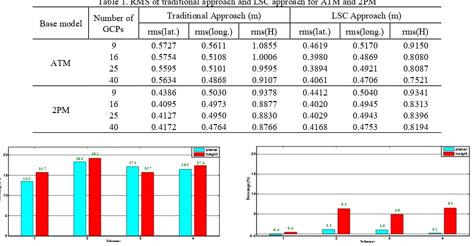
Two models (i.e., bias-corrected Affine Transformation Model (ATM) and second-order Polynomial Model (2PM)) with different number of well distributed GCPs are chosen in our numerical examples. In order to demonstrate the advantages of our LSC approach, we compute the RMS with following coordinates and the coordinates measured by GPS RTK at the CKPs, n is the number of check points, there are total 82 CKPs in our examples. Table 1 presents the RMS results of different schemes in latitude, longitude and height, both with traditional approach and LSC approach. The results show that our LSC approach can significantly improve the accuracy based on ATM, about 15 cm numerically. While the improvement based on 2PM is only about 5 cm on average in height direction.
Table 1. RMS of traditional approach and LSC approach for ATM and 2PM Base model Number of GCPs Traditional Approach (m) LSC Approach (m)
rms(lat.) rms(long.) rms(H) rms(lat.) rms(long.) rms(H)
Fig. 2. Improved percentage of LSC approach based on ATM
1 2 3 4
Fig. 3. Improved percentage of LSC approach based on 2PM
International Archives of the Photogrammetry, Remote Sensing and Spatial Information Sciences, Volume XXXIX-B1, 2012 XXII ISPRS Congress, 25 August – 01 September 2012, Melbourne, Australia
1 2 3 4 -4
0 4 8 12 16
Schemes
Pe
rc
en
ta
ge
s(%
)
planar height
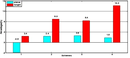
-3.9
2.4 2.4 9.0
2.6 8.4
1.8 14.2
Fig. 4. Improved percentage of LSC approach based on ATM with respect to traditional approach based on 2PM Furthermore, two histogram figures, i.e. Fig. 2 and Fig. 3, present the improved percentages of RMS in planar and height directions of LSC approach with respect to traditional approach. And Fig. 4 demonstrates the improved percentage of LSC approach for ATM compared to traditional second-order polynomial model, which shows that LSC approach for ATM can obtain even better results than traditional second-order polynomial model. As shown in Fig.2, the average improved percentages of LSC for ATM are more than 15% in both height and planar directions for different schemes. However, the improved percentages of LSC approach for 2PM in Fig. 3 are much smaller; the average result is about 5% only in height direction.
5. CONCLUDING REMARKS
This paper has put forward a LSC approach for geopositioning of HRSI, and tested it with a pair of QuickBird imagery. The results show that the geopositioning accuracy can be significantly improved with our LSC approach no matter based on ATM or 2PM. The improvements of RMS are about 15 cm in both planar and height direction based on ATM and about 5 cm in height direction based on 2PM, the correspondent percentages are about 15% and 5% on average. In addition, although the experiments are based on QuickBird imagery, the proposed LSC approach is also suitable for any types of remote sensor imagery, such as IKONOS, GeoEye, et al.
ACKNOWLEDGEMENT
This paper is largely sponsored by National key Basic Research Program of China (973 Program, Projects: 2012CB957703) and the Natural Science Foundation of China (Projects: 41074018), and partly supported by Kwang-Hua Fund for College of Civil Engineering, Tongji University.
REFERENCES
Dowman, I., Dolloff, J.T., 2000. An evaluation of rational functions for photogram-metric restitution. In: The International Archives of Photogrammetry and Remote Sensing, Amsterdam, The Netherlands, Vol. XXXIII, PartB3/1, pp. 252-266.
Dial, G., Grodecki, J., 2002. Block adjustment with rational polynomial camera models. In: Proceedings of APSRS 2002 Annual Conference, Washington D C, 22-26 April, (on CDROM).
Fraser, C.S., Hanley, H.B., 2003. Bias compensation in rational functions for IKONOS satellite imagery.
Photogrammetric Engineering & Remote Sensing, 69 (1), pp. 53-58.
Fraser, C.S., Dial, G., Grodecki, J., 2006. Sensor orientation via RPCs. ISPRS Journal of Photogrammetry and Remote Sensing 60(3), pp. 182-194.
Koch, K.R., 1977. Least squares adjustment and collocation. Bull Géod, 51, pp. 127-135.
Li B.F., Shen Y.Z., Lou L.Z., 2011. Efficient Estimation of Variance and Covariance Components: A Case Study for GPS Stochastic Model Evaluation, IEEE TRANSACTIONS ON
GEOSCIENCE AND REMOTE SENSING, 41(1), pp. 203-210
Madani, M., 1999. Real-time sensor-independent positioning by rational functions. In: Proc. of ISPRS Workshop on Direct versus Indirect Methods of Sensor Orientation, Barcelona, Spain, 25-26, November, pp. 64-75.
Rao C.R., 1971. Estimation of variance and covariance components—MINQUE theory. J Multivariate Anal 1. pp. 257–275
Tao, C.V., Hu, Y., 2002. 3D reconstruction methods based on the rational function model. Photogrammetric Engineering & Remote Sensing, 68(7), pp. 705-714
Tong, X.H., Liu, S.J., Weng, Q.H., 2010. Bias-corrected rational polynomial coefficients for high accuracy geo-positioning of QuickBird stereo imagery. ISPRS Journal of Photogrammetry and Remote Sensing, 65(1), pp. 218-226. Yang, Y., Zeng, A., Zhang, J., 2009. Adaptive collocation with application in height system transformation. J Geod, 83(5), pp. 403-410.
International Archives of the Photogrammetry, Remote Sensing and Spatial Information Sciences, Volume XXXIX-B1, 2012 XXII ISPRS Congress, 25 August – 01 September 2012, Melbourne, Australia