CALIBRATION OF THE SR4500 TIME-OF-FLIGHT CAMERA FOR OUTDOOR MOBILE
SURVEYING APPLICATIONS: A CASE STUDY
C. Heinkel´e∗, M. Labb´e, V. Muzet, P. Charbonnier
Cerema Est, Laboratoire de Strasbourg, 11 rue Jean Mentelin, B.P. 9, 67035 Strasbourg, France {Christophe.Heinkele,Valerie.Muzet,Pierre.charbonnier}@cerema.fr, [email protected]
Commission V, WG V/3
KEY WORDS:SR4500, ToF Cameras, Calibration, Outdoor dynamic acquisitions
ABSTRACT:
3D-cameras based on Time-of-Flight (ToF) technology have recently raised up to a commercial level of development. In this contribu-tion, we investigate the outdoor calibration and measurement capabilities of the SR4500 ToF camera. The proposed calibration method combines up-to-date techniques with robust estimation. First, intrinsic camera parameters are estimated, which allows converting ra-dial distances into orthogonal ones. The latter are then calibrated using successive acquisitions of a plane at different camera positions, measured by tacheometric techniques. This distance calibration step estimates two coefficient matrices for each pixel, using linear regression. Experimental assessments carried out with a 3D laser-cloud after converting all the data in a common basis show that the obtained precision is twice better than with the constructor default calibration, with a full-frame accuracy of about 4 cm. Moreover, estimating the internal calibration in sunny and warm outdoor conditions yields almost the same coefficients as indoors. Finally, a test shows the feasibility of dynamic outdoor acquisitions and measurements.
1. INTRODUCTION
In this contribution, we study the metrological performance (setup and calibration) and the measurement capacities of a recent Time-of-Flight (ToF) camera, namely the SR4500, in the context of outdoor mobile surveying applications.
Range cameras have become considerably popular in the last de-cades, thanks to their ability to simultaneously acquire a range map and an intensity matrix, at a low cost and video frame rate. Thanks to the progress of technologies, they have raised up to a commercial level of development and are now routinely used in many applications, such as robotics, medicine, automobile or video gaming. Nowadays, industrial 3D cameras offer a cheap al-ternative, albeit less accurate, to laser scanners for short-range 3D surveying in controlled environments. However, the recent appli-cation of range cameras to outdoor 3D surveying at longer ranges (Chiabrando and Rinaudo, 2013, Lachat et al., 2015) raises the question of their metrological capabilities.
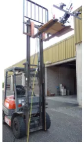
Range cameras based on ToF technologies have recently encoun-tered an increasing attention, see e.g. (Piatti et al., 2013). Sev-eral industrial sensors were developed since the seminal work of (Lange, 2000), see e.g. (Piatti and Rinaudo, 2012) for a survey. In this contribution, we consider a phase modulated (or indirect ToF) camera, namely the SR4500 (Fig. 1), launched in 2014 and manufactured by Mesa Imaging (recently acquired by the Hep-tagon company). The sensor operates in the close infrared. It is an in-pixel photomixing device (Pancheri and Stoppa, 2013), i.e. it operates a demodulation of the received optical signal for each pixel.
While the former versions of the camera were limited to 5 meters, the SR4500 has the advantage of measuring up to 10 m, depend-ing on the acquisition frequency (frequencies may be set between 15 and 30 MHz). The integration time may be set in the range [0.3-25.8] ms. Its resolution is 176×144 pixels, for a field of
∗Corresponding author
Figure 1. Picture of the SR4500 ToF camera
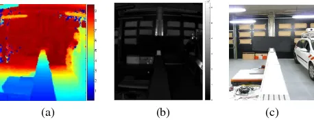
view of 69◦×55◦. A sample acquisition is shown on Fig. 2. The scene is taken in a technical hall, with an optical bench and a test vehicle. Its depth varies from 0 to 10 m. The left image shows the depth map (in false colors), where the depth gradient along the bench is clearly visible, along with some noisy pixels. The center image is the intensity image in the infrared which is, of course, slightly different from the rightmost photograph.
(a) (b) (c)
Figure 2. Sample acquisition of an indoor scene by the SR4500 ToF camera. (a) Distance matrix (b) amplitude matrix, in the close infrared (c) Photograph of the scene taken by an external camera
In this paper, we first propose an introduction to the SR4500 cam-era and its behaviour (Sec. 2). It is clear that raw measurements are not accurate enough so a calibration is needed. In the lit-erature, several publications report works on the calibration and metrological assessment of ToF cameras (in particular, of previ-ous versions of SR cameras), see e.g. (Kahlmann et al., 2006, Jaakkola et al., 2008, Robbins et al., 2008, Chiabrando et al., 2009, Lefloch et al., 2013). Inspired by these papers, we intro-duce in Sec. 3 a two-step calibration methodology. Sec. 4 is dedi-cated to an experimental assessment of this method in laboratory and outdoor conditions. Finally, Sec. 5 is a feasibility study of dynamic outdoor acquisitions and measurements.
2. BEHAVIOUR OF THE SR4500 CAMERA
2.1 Measurement principle
The SR4500 processes each pixel using the continuous wave in-tensity modulation method, which is based on the correlation be-tween the emitted signal and the received one (Lange, 2000). The emitted light being sinusoidal, with a fixed frequencyf, the cor-relation function can be written, atτ = 2πf t, as (Lefloch et al., 2013):
cτ =A0+
A
2 cos(τ+ϕ) (1)
whereAis the amplitude of the signal,A0is the offset andϕis
the phase shift between the emitted and received waves. Since there are 3 unknowns, at least 3 values are needed to calculate these parameters. Typically, 4 samples are used, at specific phase values,τ= 0, π/2, π,3π/2, as illustrated in Fig. 4.
Figure 3. Overview of phase determination technique
The phase, amplitude and offset parameters are respectively given by:
use an acquisition frequency of 15 MHz, for which the maximal reachable distance is 10 m, which is well suited to our applica-tion.
In the SR4500, 4 separate integration periods are needed to take the 4 samples that are necessary for phase measurement (Mesa Imaging AG, n.d.). The total time required to capture a depth image is hence 4 times the integration time (i.e. the time inter-val during which intensities are collected by the sensor) plus the readout time (i.e. the amount of time required to read the values). While the readout time is incompressible (about 4.6 ms for the SR4500), the integration time is a parameter, which can strongly influence distance measurements. Too high values may lead to saturation effects, while too low ones may cause noise. More-over, it was shown in (Kahlmann et al., 2006) and (Pfeifer et al., 2013) that the integration time may result in distance errors in the order of 10 cm. However, application-based constraints can influ-ence the way this value is set. In our case, dynamic acquisitions are envisioned, so short integrations times are needed to avoid motion blur and typical values of 3.3 to 10 ms will be taken.
2.2 Quality of ToF data
The raw measurements provided by ToF cameras are impaired by errors of different natures. A comprehensive panorama of range-camera errors is out of the scope of this paper and we refer the reader to e.g. (Lefloch et al., 2013, Rapp, 2007) for more insight about these phenomena. In this section, we illustrate systematic and random errors on a simple example.
The repeatability of the raw data of the SR4500 was studied with 50 acquisitions of a white wall placed at 2 m of the camera. The integration time was set at 3.3 ms. The standard deviation of these 50 measures was computed for each pixel and is shown in Fig. 4. In the central part of the image, the standard deviation is between 2 and 3 cm and it reaches 9 cm in the corners. We note that these results are qualitatively similar to those obtained by Kahlman (Kahlmann et al., 2006) for a SR-2 camera.
The same experiment was done for a 10 ms integration time. With this setting, the standard deviation of the center is around 0.72 cm while it is 4 cm on the borders. We observe that the standard deviation decreases when the integration time is bigger. This is in accordance with the variation law of the variance with respect to the inverse of the squared amplitude exhibited by Rapp in (Rapp, 2007).
This example illustrate the need for correcting measurement er-rors. To reduce the effect of random errors, averages are often used. However, it is most of the time preferable to use more robust estimators, such as the median, for example. Systematic measurement errors may be addressed by calibration.
2.3 Internal heating time and integration time
Figure 4. Standard deviation (m) of 50 acquisitions (sight dis-tance of 2 m, integration time of 3.3 ms)
20 40 60 80
Figure 5. Evolution of the measured distance (left) and standard deviation (right) with time for different acquisition times
a sight distance of 3.5 m for 4 different integration time: 3.3, 5.3, 10 and 20 ms. For each integration time, 50 acquisitions were taken every 5 min and we studied the raw data given by the Mesa software. The median and the standard deviation are presented for the central part of the image (30×24 pixels) in Fig. 5. The measured distance almost corresponds to the real distance at 3.3 and 5.5 ms while there is an important distance offset at 10 and 20 ms. Since the default value of the Mesa SR4500 integration time is 3.3 ms (Mesa Imaging AG, n.d.), it seems that the default calibration corresponds to this setting. For the longest integration times of our study (10 and 20 ms), during the first 20 minutes of heating, the variation of the measured distance reaches 4 cm. At an acquisition time of 3.3 ms, there is less variation of the median distance but the standard deviation needs more time to reach sta-bility (40 to 60 minutes). Hence, a heating time of 40 min at least was systematically respected in all our experiments.
This experiment confirms the need for a correction of distances. Clearly, this calibration must be adapted to each integration time setting.
3. CALIBRATION METHODOLOGY
Sources of systematic error are many in range imaging, see e.g. (Lefloch et al., 2013). In such a context, substantial gains in pre-cision are accessible using calibration techniques. In this section,
Figure 6. Transforming a radial distance into an orthogonal dis-tance, following (Rapp et al., 2008)
Figure 7. Photographs of the calibration checkerboard installed indoors (a) and outdoors (c); corresponding amplitude images output by the SR4500 indoors (b) and outdoors(d)
we recall the basis ideas of the two calibration procedures we use. The first one, internal, or lateral (Lindner and Kolb, 2006), cali-bration aims at transforming the radial distance provided by the range camera into an orthogonal distance, or depth. The second one, distance or depth calibration, is used to adjust the outputs to reference measurements.
3.1 Internal calibration
As for ordinary cameras, the internal calibration of range cam-eras relies on the determination of the intrinsic parameters of the device. These camera-specific parameters are, in particular, the focal lengthf, the optical image center(cx, cy), the pixel size and the distortion coefficients. Once these parameters are esti-mated, it is possible to compensate for distortions caused by the sensor lens, but also to convert any radial distanceDradinto an orthogonal oneDorthusing the pin-hole model, as described e.g. in (Rapp et al., 2008), see Fig. 6. The transformation is governed by the following relationship:
The second step consists of the calibration of the orthogonal dis-tances obtained from eq. (6). Successive images of a plane sur-face are taken with the SR4500 at different distances, as illus-trated on Fig. 8. These reference distances are measured with a very accurate system (such as laser scanners, tacheometers (Chiabrando et al., 2009) or linear positionner tables (Rapp, 2007)).
Figure 8. Scheme of the distance calibration method: reference distances are drawn in blue and SR4500 outputs are in red
In this work, we perform a per-pixel linear calibration. In other words, a linear regression is computed for each pixel, to adjust the data given by the camera to the reference distances. The out-put of the procedure is hence a pair of 25344-element matrices: one for the slopes and one for the offsets. Other techniques might be used, such as lookup tables (Kahlmann et al., 2006), but lin-ear adjustment is more storage-efficient, as noticed in (Lindner and Kolb, 2006). While more sophisticated models, involving B-spline global correction (Lindner and Kolb, 2006) or polynomial regression (Schiller et al., 2008), might be envisioned, we found that the linear model was a good compromise between accuracy and complexity for our applications.
4. EXPERIMENTAL CALIBRATIONS
In this section, we propose an experimental assessment of the calibration methodology in both indoor and outdoor conditions.
4.1 Internal calibration
The calibration checkerboard has been used indoors and outdoors. In the indoor setting it is fixed on a wall and the camera is placed on a tripod; outdoors, it is laid on the floor and the SR4500 is attached to a forklift as depicted on Fig. 9. Figure 10 shows the position and orientation of the views taken in both situations.
Table 1 shows a comparison of the intrinsic parameters obtained in both configurations. Although the uncertainties provided by Bouguet’s toolbox significatively increased outdoors, the differ-ences of the computed parameters are quite small.
Despite the experimental conditions were not perfect (in partic-ular, the ground is not really plane), this experiment shows the feasibility of an internal calibration outdoors, which might be of a great interest for future applications.
Figure 9. The SR4500 is fixed on a forklift for outdoor internal calibration
Figure 10. Orientation of the camera during indoor calibration (top) and outdoor calibration (bottom)
Indoor calibration Outdoor calibration values uncertainties values uncertainties
fx 10.09 0.09 10.08 0.18
fy 10.09 0.08 10.08 0.19
cx 3.61 0.12 3.62 0.11
cy 2.65 0.11 2.72 0.17
4.2 Distance calibration
The calibration of the orthogonal distances is computed from successive acquisitions of a plane for different camera positions. These successive planes (Fig. 8) are obtained by moving the cam-era and making acquisition of a wall. At each scanning position, two Trimble M3 tachometers with a measurement precision of 3 mm are used for locating the camera and measuring its dis-tance from the observed wall. To make the absolute localisation of the SR4500 ToF camera easier, several stickers are applied on it (see Fig. 11). To find the stickers coordinates and the checker-boards centres in the world scene, the tachometer data are pro-cessed with the Autocad COVADIS plug-in. Four checkerboards are also placed on the wall (Fig. 12) and their four centers are acquired by each tachometer.
Figure 11. Stickers applied on the SR4500 camera to facilitate its localisation with the tachometer
Figure 12. View of the calibration wall and the 2 tachometers
At each of 22 scanning position, 50 images are taken by the SR4500 with a 3.3 ms integration time and their median is com-puted. These data are then used for per-pixel linear regression with respect to the reference plane positions.
A crucial point for the method is to measure the reference planes accurately. Once 3 points on the camera and 3 points on the wall are known in world coordinates, it is possible to estimate the 3D Helmert transformation between the camera and the refer-ence plane. However, the stickers applied on the ToF camera are too close to each others, and the obtained precision is not suffi-cient, especially on the rotational components of the transform. Fig. 13(a) shows that the reference and measured planes, that should be parallel, are indeed secant. To fix the reference plane orientation problem, we estimate the rotational components using the normal to each plane. Since the SR4500 data are very noisy, the normal to the camera point cloud is estimated using a robust Principal Component Analysis (PCA) algorithm, see (Moisan et al., 2015) for more details.
Once the orientation is corrected, the planes are parallel, as shown
(a) (b)
Figure 13. Point cloud of the calibration plane generated by the camera (in blue) and reference plane (in red). (a) obtained by Helmert 3D transformation (b) after alignment of the normal to the planes
in Fig. 13(b). Finally, a linear regression is performed on each pixel between the reference planes and the ToF camera cloud. As planned, the regression is linear and 2 matrices of144×176 = 25344coefficients are computed, one for the slope and one for the offset. After applying these coefficients to each acquisition, a depth map is computed for each acquisition distance.
4.3 Accuracy and dispersion assessments
In order to assess the quality of our calibration, a very accurate survey of the wall was performed using a FarorFocus3D. The
resolution of the resulting geo-referenced point cloud is 2 mm. It is then down-sampled to the SR4500 resolution. The Root-Mean-Square (RMS) deviation is computed between the refer-ence FARO plane and the depth maps. Fig. 14 shows the RMS deviation as a function of the sight distance, for both the depth maps provided by the Mesa-Imaging software, which uses the internal default calibration of the camera, and the depth maps obtained by our method. The accuracy is about 4 cm with our calibration and 6 cm for the Mesa output.
To estimate the dispersion of the data points, a plane is first ad-justed to the depth maps by robust PCA and the standard devia-tion of the depths with respect to this plane is computed. Fig. 15 shows the obtained precision as a function of the sight distance, for the Mesa-imaging depth maps and the results of our method. At 4.96 m, the mean standard deviation obtained with our cali-bration is±1.6 cm instead of±3.3 cm for the default calibration. The proposed method reduces systematic errors better than the Mesa-Imaging software.
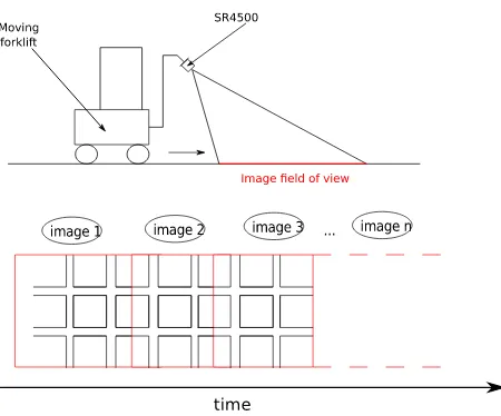
5. FIRST ATTEMPT AT OUTDOOR DYNAMIC ACQUISITIONS
Since our laboratory results were satisfactory, a dynamic acqui-sition test was performed outdoors, at slow motion. The object we survey is a white grid (with spacing 1 m±2 cm) painted on a contrasting road surface, with an almost horizontal profile (see Fig. 16). For practical reasons, the acquisitions were performed with the constructor software SR3DView and, in this first ap-proach, we used the default calibration given by Mesa.
5.1 Experimental set-up
5
6
7
8
9
0
Sight distance (m)
RMS
(a)
5
6
7
8
9
0
2
4
6
·
10
−2Sight distance (m)
RMS
de
viation
(m)
(b)
Figure 14. RMS deviation (accuracy) at different observation dis-tances (a) between the depth maps obtained by Mesa-Imaging software and the Faro plane, (b) between the corrected depths ob-tained with our distance calibration and the FARO plane
0 2 4 6 8
0 2 4 6 ·10
−2
Sight distance (m)
Standard
de
viation
(m)
(a)
0 2 4 6 8
0 2 4 6 ·10
−2
Sight distance (m)
Standard
de
viation
(m)
(b)
Figure 15. Standard deviation (precision) at different observation distances for (a) the Mesa-Imaging software (b) our calibration method
The image recording was done while the forklift moved at about 4 km.h−1
.
Figure 16. Picture of the surface of interest
Figure 17. Sketch of the experimental outdoor set-up in dynamic
5.2 Points cloud processing
The point clouds provided by the camera are very noisy, as can be seen on Fig. 18. However, they can be easily enhanced by taking advantage of prior information about the scene and accounting for the amplitude image. Indeed, most flying pixels correspond to low amplitudes, so they can be eliminated by a simple thresh-old. The remaining outliers are filtered out after fitting the ground plane using robust PCA.
Figure 18. Point cloud of one acquisition of the grid. Point colors depict the amplitude signal. Outliers pixels are mostly located on a plane above the road
Figure 19. Full grid point cloud reconstructed by successive ICP
To assess the feasibility of dimensional measurements in these conditions we calculate the size of the grid marking. Since the contrast between the marking and the asphalt is important, the scalar information of the amplitude image output by the ToF cam-era can be used. The marking is segmented using an arbitrary threshold. Then, rectangles are adjusted in 3D using some se-lected points, see 20. Their sizes can be compared with the phys-ical size of the marking, as shown on Tab. 2 (the theoretphys-ical size is 19×81 cm).
Figure 20. Extraction of several rectangles (successively colored in violet, green, blue, orange, pink and black) from the SR4500 point cloud that correspond to the marking
Colour Width (cm)×length (cm)
violet 16×81
Table 2. Measured size of marking extracted from the local planes represented in colours on figure 20
With this methodology, the precision of marking sizes is around 2 cm, which corresponds to the precisions of the grid. Since the data were taken at low speed, under a high sun illumination, and without specific calibration, these results are promising.
6. CONCLUSION
In this paper, we first presented the two calibration steps of the SR4500 ToF camera. The internal calibration was done indoors and outdoors, whereas the distance calibration was performed only indoors. Our experimental full-frame assessments show an accuracy of about 4 cm with a precision of 1.6 cm at 5 m.
This study reveals a very good behaviour of the SR4500 outdoors, even in hot temperature conditions and high illumination level.
The internal camera parameters estimated in these sunny condi-tions are similar to those obtained indoors. A perspective of the present work could be to perform a distance calibration outdoors with a scanner laser acquisition of the whole scene at each camera position. With this setup, the reference could be more accurate and better accuracies may be expected.
Finally, the experiments show the feasibility of using the SR4500 ToF Camera outdoors even for dynamic applications, albeit the speed was limited in our experiments. Up to now, the ToF Camera cloud are processed manually. Further experiments in dynamic conditions will need more automated processes.
REFERENCES
Besl, P. and McKay, N. D., 1992. A method for registration of 3-D shapes.IEEE Transactions on Pattern Analysis and Machine Intelligence, 14(2), pp. 239–256.
Bouguet, J.-Y., 1999. Camera Calibration Toolbox for Matlab, http://www.vision.caltech.edu/bouguetj/calib doc/index.html. Accessed April 2016.
Chiabrando, F. and Rinaudo, F., 2013. TOF Cameras for Archi-tectural Surveys. In: F. Remondino and D. Stoppa (eds), TOF Range-Imaging Cameras, Springer Berlin Heidelberg, Berlin, Heidelberg, pp. 139–164.
Chiabrando, F., Chiabrando, R., Piatti, D. and Rinaudo, F., 2009. Sensors for 3D imaging: metric evaluation and calibration for a CCD/CMOS time-of-flight camera. Sensors, 9, pp. 10080– 10096.
Jaakkola, A., Kaasalainen, S., Hyypp¨a, J., Akuj¨arvi, A. and Niit-tym¨aki, H., 2008. Radiometric calibration of intensity images of swissranger SR-3000 range camera. The photogrammetric jour-nal of Finland, 21(1), pp. 16–25.
Kahlmann, T., Remondino, F. and Ingensand, H., 2006. Calibra-tion for increased accuracy of the range imaging camera Swis-sranger. In: H.-G. Maas and D. Schneider (eds),Proceedings of the ISPRS Commission V Symposium ’Image Engineering and Vision Metrology’, IAPRS Volume XXXVI, Part 5, Dresden, Ger-many, pp. 136–141.
Lachat, E., Macher, H., Mittet, M.-a., Landes, T. and Grussen-meyer, P., 2015. First Experiences With Kinect V2 Sensor for Close Range 3D Modelling. ISPRS - International Archives of the Photogrammetry, Remote Sensing and Spatial Information Sciences, XL-5/W4(February), pp. 93–100.
Lange, R., 2000. 3D time-of-flight distance measurement with custom solid-state image sensors in CMOS/CCD-technology. PhD thesis, Siegen.
Lefloch, D., Nair, R., Lenzen, F., Schaefer, H., Streeter, L., Cree, M. J., Koch, R. and Kolb, A., 2013. Time-of-Flight and Depth Imaging. Sensors, Algorithms, and Applications. Vol. 8200, Springer Berlin Heidelberg, chapter Technical Foundation and Calibration Methods for Time-of-Flight Cameras, pp. 3–24.
Lindner, M. and Kolb, A., 2006. Lateral and Depth Calibra-tion of PMD-Distance Sensors. Advances in Visual Computing, 4292(4292/2006), pp. 524–533.
Pancheri, L. and Stoppa, D., 2013. TOF Cameras for Architec-tural Surveys. In: F. Remondino and D. Stoppa (eds),Sensors based on in-pixel photomixing devices, Springer Berlin Heidel-berg, Berlin, HeidelHeidel-berg, pp. 69–90.
Pfeifer, N., Lichti, D., B¨ohm, J. and Karel, W., 2013. 3D Cam-eras: Errors, Calibration and Orientation. In: F. Remondino and D. Stoppa (eds),TOF Range-Imaging Cameras, Springer Berlin Heidelberg, pp. 117–138.
Piatti, D. and Rinaudo, F., 2012. SR-4000 and camcube3.0 time of flight (ToF) cameras: Tests and comparison. Remote Sensing, 4, pp. 1069–1089.
Piatti, D., Remondino, F. and Stoppa, D., 2013. TOF Cameras for Architectural Surveys. In: F. Remondino and D. Stoppa (eds), State-of-the art of TOF Range-Imaging sensors, Springer Berlin Heidelberg, Berlin, Heidelberg, pp. 1–10.
statistical uncertainties of Time-Of-Flight-cameras.International Journal of Intelligent Systems Technologies and Applications, 5, pp. 402–413.
Robbins, S., Schroeder, B., Murawski, B., Heckman, N. and Le-ung, J., 2008. Photogrammetric calibration of the swissranger 3D range imaging sensor. In:Proceedings of SPIE, Vol. 7003number 700320, SPIE Digital Library.