AUTOMATIC 3D MAPPING
USING MULTIPLE UNCALIBRATED CLOSE RANGE IMAGES
M. Rafiei, M. SaadatsereshtDepartment of Surveying Engineering, University of Tehran, Iran (meysam.rafiei, msaadat)@ut.ac.ir
KEY WORDS: Close Range Photogrammetry, Automatic, 3D mapping, Euclidean Reconstruction, Uncalibrated Images
ABSTRACT:
Automatic three-dimensions modeling of the real world is an important research topic in the geomatics and computer vision fields for many years. By development of commercial digital cameras and modern image processing techniques, close range photogrammetry is vastly utilized in many fields such as structure measurements, topographic surveying, architectural and archeological surveying, etc. A non-contact photogrammetry provides methods to determine 3D locations of objects from two-dimensional (2D) images. Problem of estimating the locations of 3D points from multiple images, often involves simultaneously estimating both 3D geometry (structure) and camera pose (motion), it is commonly known as structure from motion (SfM). In this research a step by step approach to generate the 3D point cloud of a scene is considered. After taking images with a camera, we should detect corresponding points in each two views. Here an efficient SIFT method is used for image matching for large baselines. After that, we must retrieve the camera motion and 3D position of the matched feature points up to a projective transformation (projective reconstruction). Lacking additional information on the camera or the scene makes the parallel lines to be unparalleled. The results of SfM computation are much more useful if a metric reconstruction is obtained. Therefor multiple views Euclidean reconstruction applied and discussed. To refine and achieve the precise 3D points we use more general and useful approach, namely bundle adjustment. At the end two real cases have been considered to reconstruct (an excavation and a tower).
1. INTRODUCTION
There are many ways to mapping and obtain 3D models of the world around us and every approach has some advantage and disadvantage. In this regard some approaches are automatic, semi-automatic and some are automatic. Mostly non-automatic and semi-non-automatic manners are time-consuming, costly and need more than one operator. On the other hand, automatic approaches are very fast, simple and need one operator to perform. One of these methods is Close Range Photogrammetry. Digital close range photogrammetry is a low-cost technique for accurately measuring objects directly from digital images captured with a camera at close range.
Image-based modeling uses digital cameras and requires a mathematical formulation to transform 2D image coordinates into 3D information. Images contain all the useful information to form geometry and texture for a 3D modeling application (Luigi Barazzetti et al., 2010). Automatic techniques can be used to track the image features and solve it mathematically by using Structure from Motion (SfM) techniques, which refer to the computation of the camera stations and viewing directions (imaging configuration) and the 3D object points from at least two images (Alsadik et al., 2012).
Most of earlier studies in this field assume that the intrinsic parameters of the camera (focal length, image center and aspect ratio) are known. Computing camera motion in this case is a
well-known problem in photogrammetry, called relative orientation (Atkinson, 1996). Some of them (Boufama et al., 1993) put some constraints on the reconstruction data in order to get reconstruction in the Euclidean space. Such constraints arise from knowledge of the scene: location of points, geometrical constraints on lines, etc. The paper of Barazzetti et al (2010) focused on calibrated camera. Cronk et al (2006) used coded targets for the calibration and orientation phase. Targets are automatically recognized, measured and labeled to solve the identification of the image correspondences. This solution becomes very useful and practical, but in many surveys targets cannot be used or stick at the object.
2. THEORY
2.1 Image Matching
Features such as points and edges may change dramatically after image transformations, for example, after scaling and rotation. As a result, recent works have concentrated on detecting and describing image features that are invariant to these transformations. Scale Invariant Feature Transform (SIFT) is a feature-based image matching approach, which lessens the damaging effects of image transformations to a certain extent. Features extracted by SIFT are invariant to image scaling and rotation, and partially invariant to photometric changes. SIFT mainly covers 4 stages throughout the computation procedure as follows (D. Lowe, 2004):
1. Local extremum detection: first, use difference-of-Gaussian (DOG) to approximate Laplacian-of-difference-of-Gaussian and build the image pyramid in scale space. Determine the keypoint candidates by local extremum detection.
2. Strip unstable keypoints: use the Taylor expansion of the scale-space function to reject those points that are not distinctive enough or are unsatisfactorily located near the edge.
3. Feature description: Local image gradients and orientations are computed around keypoints. A set of orientation, scale and location for each keypoint is used to represent it, which is significantly invariant to image transformations and luminance changes.
4. Feature matching: compute the feature descriptors in the target image in advance and store all the features in a shape-indexing feature database. To initiate the matching process for the new image, repeat steps 1-3 above and search for the most similar features in the database.
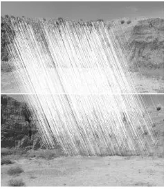
SIFT has been shown to be a valuable tool in 3D reconstruction. In this context (3D mapping) we face with large baseline in image acquisition stations. Some stations are near the object, the others are far from it probably. There is no smoothness in camera stations. In addition, rotation of camera is not like the aerial photography. Most the time the rotation matrix has large components. On the other hand, keypoints extracted by SIFT are highly distinctive so that they are invariant to image transformation and partially invariant to illumination and camera viewpoint changes. So we prefer to use SIFT method for feature extraction and feature matching steps. Figure 1 shows efficiency of the SIFT in image matching process.
2.2 The Camera Model
The projection of a point in space with coordinates X onto the image plane has (homogeneous) coordinates x' that satisfy the equation (1).
[ ] (1)
Figure 1. Efficiency of the SIFT in image matching
where [ ] and is the pose of the camera in the (chosen) world reference frame. In the equation above, the matrix K, which is define as
[ ] , (2)
describes “intrinsic” properties of the camera, such as the position of the optical center ( ), the size of the pixel ( ), its skew factor , and the focal length f. The matrix K is called the intrinsic parameter matrix, or simply calibration matrix, and it maps metric coordinates (units of meters) into image coordinates (units of pixels). In what follows, we denote pixel coordinates with a prime superscript , whereas metric coordinates are indicated simply by . The rigid-body motion represents the “extrinsic” properties of the camera, namely, its position and orientation relative to a chosen world reference frame. The parameters are therefore called extrinsic calibration parameters.
2.3 The Fundamental Matrix F
The fundamental matrix is the algebraic representation of epipolar geometry. The fundamental matrix maps, or
“transfers”, a point in the first view to a vector l2 F in the second view via
F = l2 = 0.
In fact, the vector l2defines implicitly a line in the image plane as the collection of image points { } that satisfy the equation
Given at least 8 correspondence, F can be estimated using the linear eight-point algorithm. If the number of correspondence was more than 8, a nonlinear algorithm should be used. Most of time, there are outliers in process of establishing correspondence and estimating F. These outliers eliminate in step of estimating the fundamental matrix simultaneously using RANSAC.
2.4 Projective Reconstruction
projective transformation could be directly recovered. In the absence of any additional information, this is the best one can do. We start with the case of two views, and use the results to initialize a multiple-view algorithm (Yi Ma, et al., 2003).
2.4.1 Two View Initialization: The generic point p
Recovering Projection Matrices and Projective Structure: Given the fundamental matrix F estimated via 8-point algorithm, there are several ways to decompose it in order obtain projection matrices and 3D structure from the two views. Since F = ̂ , all projection matrices [
] yield the same fundamental matrix for any value of
[ ] and , and hence there is a four-parameter family of possible choices. One common choice, known as the canonical decomposition, has the following form
[ ] [( ̂) ]
( ̂)
Now, different choices of and result in different projection matrices , which in turn result in different projective coordinates Xp, and hence different reconstructions. Some of these reconstructions may be more “distorted” than others, in the sense of being farther from the “true” Euclidean reconstruction. In order to minimize the amount of projective distortion and obtain the initial reconstruction as close as possible to the Euclidean one, we can play with the choice of and , as suggested in (Beardsley et al., 1997). In practice, it is common to assume that the optical center is at the center of the image, that the focal length is roughly known (for instance from previous calibrations of the camera), and that the pixels are square with no skew. Therefore, one can start with a rough approximation of the intrinsic parameter matrix K, call it ̃. After doing so, we can choose and by requiring that the first block of the projection matrix be as close as possible to the rotation matrix between two views, ( ̂) . In case the actual rotation R between the views is small, we can start by choosing ̃ I, and solve linearly for and . In case of general rotation, one can still solve the equation
( ̂) for , provided a guess for the rotation ̃ is available. When the projection matrices, and have chosen, the 3D structure can be recovered. Ideally, if guess of ̃ was accurate, all points should be visible; i.e. all estimated scales should be positive. If this is not the case, different values for the focal length can be tested until the majority of points have camera poses for the m views and the 3D structure of any point that appears in at least two views. For convenience, we will use the same notation [ ] with and .
The core of the multiple-view algorithm consists of exploiting the following equation, derived from the multiple-view rank conditions:
This leads to an algorithm which alternates between estimation of camera motion and 3D structure, exploiting multiple-view constraints available in all views. After the algorithm has converged, the camera motion is given by [ ], i= 2,3, . . . ,m, and the depth of the points (with respect to the first camera frame) is given by , j= 1,2, . . . ,n. The resulting projection matrices and the 3D structure obtained by the above iterative procedure can be then refined using a nonlinear optimization called reprojection error.
∑ ∑ ‖ ‖ (6)
If the reprojection error is still large, the estimates can be refined using a nonlinear optimization procedure that simultaneously updates the estimates of both motion and structure parameters.
2.5 Upgrade From Projective To Euclidean Reconstruction
The projective reconstruction obtained in the absence of calibration information, is related to the Euclidean structure
by a linear transformation ,
(7)
Where indicates equality up to a scale factor, [ ] and H has the form
2.5.1 Stratification With The Absolute Quadric Constraint: According to the equation
[ ]
where we use [ ]to denote the Euclidean motion between the ith and the first camera frame. Since the last column gives three equations, but adds three unknowns, it is useless as far as providing constraints on H. Therefore, we can restrict our attention to the leftmost 3×3 block
[ ] (9)
One can then eliminate the unknown rotation matrix by multiplying both sides by their transpose:
[ ] (10)
If we define , and
[
] (11)
then we obtain the absolute quadric constraint as bellow
(12)
If we assume that K is constant, so that Ki = K for all i, then we can minimize the angle between the vectors composing the matrices on the left-hand side and those on the right-hand side with respect to the unknowns, K and , using for instance a gradient descent procedure. Alternatively, it could first estimate Q and Ki from this equation by ignoring its internal structure; then, H and K can be extracted from Q, and subsequently the recovered structure and motion can be upgraded to Euclidean. Figure 2 shows the Euclidean reconstruction of a projective form.
Figure 2. Upgrade from projective to Euclidean reconstruction
2.6 Euclidean Bundle Adjustment
In order to refine the estimate obtained so far, we can set up an iterative optimization, known as Euclidean bundle adjustment, by minimizing the reprojection error as in Section 2.4.2, but this time with respect to all and only the unknown Euclidean parameters: structure, motion, and calibration. The reprojection error is still given by
∑ ∑ ‖ ‖ (13)
However, this time the parameters are given by
} , where are the exponential coordinates
of rotation ̂ and are computed via Rodrigues’ formula. The total dimension of the parameter space is 5 + 6(m - 1) + 3n for m views and n points (Yi Ma, et al., 2003).
3. IMPLEMENTATION
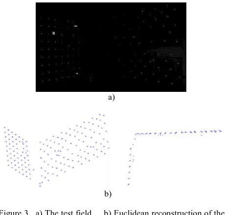
At first, we created a test field to evaluate of our approach. The test field was created from some retro-reflective targets to compare our technique with the Australis software. We used this kind of test field because it was a simple and good way to test the 3D metric reconstruction. Figure 3 shows the test field and its 3D model.
a)
b)
Figure 3. a) The test field b) Euclidean reconstruction of the test field
To implement our approach in real word, we consider two cases to reconstruct: an excavation and a historical tower. In this study, the Canon SX230 digital camera (a non-metric digital camera with Manual setting to fix the focal length) has been used (Figure 4).
Figure 4. Canon SX230 digital camera
3.1 Case Studies
Figure 5. The excavation, its 3D point clouds and model
Area of the excavation field was about 400m2. The 22 consequence images have been taken to cover all the area.
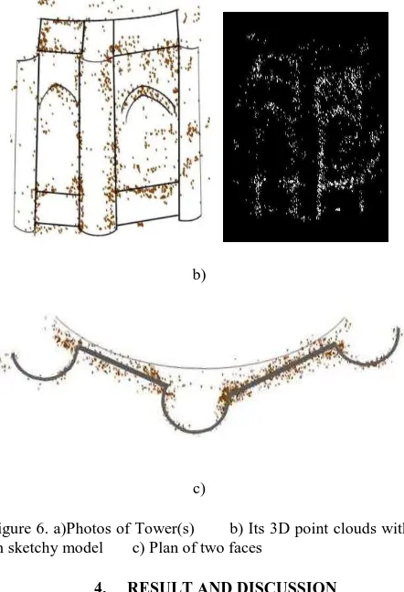
Kharraqan Towers: The need for documentation of historic buildings is greatly admitted by many experts in numerous literatures. One step in documentation is surveying or 3D modeling. In this regard, digital close range photogrammetry shows a high proficiency and it is a low-cost technique to collects 3D information about an object. The two Kharraqan Tomb Towers are located in 33km west of Ab-e Garm town, in Qazvin Province in Iran. These two towers are particularly notable for their vivid external decoration, which classes them amongst the finest decorated brick monuments found in Iran (Briseghella & Kalhor, 2007).
We consider just two sides of west tower for modeling. The model of two faces of this octagon tower has been formed with 6 images. A superficial network is designed to reach the minimum number of at least three cameras for each point (Fraser, 1989). Figure 6 shows the efficiency of this technique to reconstruct the historical tower.
a)
b)
c)
Figure 6. a)Photos of Tower(s) b) Its 3D point clouds with an sketchy model c) Plan of two faces
4. RESULT AND DISCUSSION
With the use of the test field, a comparison between our technique and Australis 3D modeling has been done. Table 1 shows the differences between each direction.
Direction X Y Z
RMS (mm) 1.3 1.5 3
Table 1. Accuracy assessment between our technique and Autralis (Z axis is in direction of first camera’s focal length)
When experimental result examined, photogrammetric technique is efficient for fast 3D mapping. The first case study modeling has been showed about 8cm differences in a one large length at a huge excavation. It is so better in Kharraqan Tower reconstruction; the difference was about 3cm.
This method has been shown that by generating dense point clouds, it is more effective than classical surveying in such volume calculation. In addition, image based modeling could approach 97.3 % ratio to the real value. On the other hand, it is a very low cost and fast technique. It reduces the land work time and usually needs one people to work, but classical land surveying needs at least 3 people to work. Consequently, photogrammetric methods have 33.33% cost advantage in field works when compared with the classical method (M.Yakar et al., 2008).
more images and it increases the computational process (in the case of partial imaging). Moreover, it leads to block error in bundle block adjustment if the images don’t have an adequate overlap (more than 60%). This is very important to select an appropriate digital camera proportional to the project. If the object is big or distance to object is large, it should be to use a camera with high resolution. It is suggested that for 3D reconstruction projects it is better to use SLR digital cameras.
5. CONCLUSION
By the development of off-the-shelf digital cameras and modern image processing techniques, digital close range photogrammetry is vastly utilized in many fields such as engineering structure measurements, topographic and archeological surveying, etc. Both cheap and fast features lead to vast use of this method.
In this research, we consider an approach to reach a three-dimensional Euclidean model of an object or a scene by means of an automatic manner. By the help of perspective projection, it is possible to goes from 2D images to 3D features. Problem of estimating the locations of 3D points from multiple images commonly known as structure from motion (SfM). We used an efficient SIFT method to solve the correspondence problem, which it is a basic step in SfM. After that to reach the metric reconstruction, we passed the projective transformation. At the end a nonlinear bundle adjustment was applied to refine the estimated obtained.
To implement the mentioned technique, we started with a test field to evaluate our technique. This kind of test field has been used to compare our approach with Australis software. The result show acceptable differences and confirm our approach for 3D metric modeling. Then for testing above, we consider an excavation and a historical tower to reconstruct. The excavation case was elected because of widely usage of this approach in such fields, and to show the performance of this method to documentation of historical places, the Kharraqan Tomb Towers was selected. To cover the two cases, respectively, 22 and 6 images have been taken for excavation and historical tower.
REFERENCES
Atkinson, K.B., 1996. Close Range Photogrammetry and Machine Vision, Whittles Publishing, Scotland.
Barazzetti, L., Scaioni, M., Remondino, F., 2010. Orientation and 3D modeling from markerless terrestrial images: combining accuracy with automation. The Photogrammetric Record 25, pp.356-381.
B. Boufama R. Mohr F. Veillon, 1993. Euclidean Constraints for Uncalibrated Reconstruction. IEEE.
Briseghella L. and M. Kalhor, 2007. The Seismic Rehabilitation of Kharraqan Tomb Towers. The 5th international conference on seismology and earthquake engineering, Tehran, Iran.
B. S. Alsadik, M. Gerke, G. Vosselman, 2012. OPTIMAL CAMERA NETWORK DESIGN FOR 3D MODELING OF CULTURAL HERITAGE. ISPRS Annals of the Photogrammetry, Remote Sensing and Spatial Information Sciences, Volume I-3, Melbourne, Australia.
Cronk, S., Fraser, C. and Hanley, H., 2006. Automated metric calibration of colour digital cameras. Photogrammetric Record, 21(116): 355–372.
Fraser, C.S., 1989. Non Topographic Photogrammetry, 2nd edition ed. Edwards Brothers Inc.
Lowe, D.G., 2004. Distinctive Image Features from Scale-Invariant Keypoints. International Journal of Computer Vision.
M.Yakar, H.M. Yilmaz, 2008. USING IN VOLUME
COMPUTING OF DIGITAL CLOSE RANGE
PHOTOGRAMMETRY, The International Archives of the Photogrammetry, Remote Sensing and Spatial Information Sciences, Vol. XXXVII. Part B3b. Beijing.