MAPPING BIOMASS AVAILABILITY TO DECREASE THE DEPENDENCY
ON FOSSIL FUELS
T. Steensen a, *, S. Müller b, M. Jandewerth c, O. Büscher b
a Institute of Photogrammetry and GeoInformation, Leibniz Universität Hannover, Germany - [email protected]
b
EFTAS Fernerkundung Technologietransfer GmbH, Münster, Germany – (soenke.mueller, olaf.buescher)@eftas.com c
Fraunhofer-Institut für Umwelt-, Sicherheits- und Energietechnik UMSICHT, Oberhausen, Germany - [email protected]
KEY WORDS: Vegetation, Satellite, LIDAR, GIS, Hyperspectral, Mapping
ABSTRACT:
To decrease the dependency on fossil fuels, more renewable energy sources need to be explored. Over the last years, the consumption of biomass has risen steadily and it has become a major source for re-growing energy. Besides the most common sources of biomass (forests, agriculture etc.) there are smaller supplies available in mostly unused areas like hedges, vegetation along streets, railways, rivers and field margins. However, these sources are not mapped and in order to obtain their potential for usage as a renewable energy, a method to quickly assess their spatial distribution and their volume is needed. We use a range of data sets including satellite imagery, GIS and elevation data to evaluate these parameters. With the upcoming Sentinel missions, our satellite data is chosen to match the spatial resolution of Sentinel-2 (10-20m) as well as its spectral characteristics. To obtain sub-pixel information from the satellite data, we use a spectral unmixing approach. Additional GIS data is provided by the German Digital Landscape Model (ATKIS Base-DLM). To estimate the height (and derive the volume) of the vegetation, we use LIDAR data to produce a digital surface model. These data sets allow us to map the extent of previously unused biomass sources. This map can then be used as a starting point for further analyses about the feasibility of the biomass extraction and their usage as a renewable energy source.
* Corresponding author. This is useful to know for communication with the appropriate person in cases with more than one author.
1. INTRODUCTION
Stepping away from fossil fuels and their related carbon dioxide (CO2) emissions requires research into new, alternative and renewable energy sources. Such resources are generated on a daily level or over short periods of time (i.e. solar influx on the earth, wind or tidal power) and have seen a substantial amount of research to evaluate their potential (see Hepbasli, 2008, for an overview). A different approach to renewable energies can be taken via biomass, which can be used for heating and electricity generation (Voivontas et al., 2001). As opposed to coal and gas, the generation of power through solar energy, wind, water or biomass does not unlock long-buried CO2 and, thus, does not effectively add CO2 to the atmosphere in the medium to long term. This lack of net-created CO2 has caused the interest in biomass in sight of the ongoing debate about climate change and the consequences for the environment (Field et al., 2007).
The high abundance of biomass, its fast regeneration and the general easy accessibility are factors in favour of it being used as a renewable energy source. Principal targets for the biomass generation are forests and agricultural areas but, with the growing urbanisation, their extent is more and more limited and alternative vegetation sources need to be found.
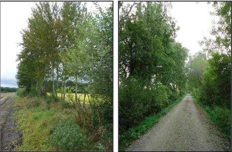
In this study, we focus on alternate biomass sources that have been largely ignored in the past. These targets include vegetation strips alongside streets, railways and waterways, unploughed strips that separate fields as well as hedges in general (see Figure 1 for examples). The object areas generally
have elongated shapes with a limited width in the range of 5 to 20m. The location of these vegetation types can be in bucolic as well as urban areas allowing for a wide range of potential biomass energy.
Figure 1. Examples of the vegetation used in our study: unploughed strips (left) and vegetation alongside streets (right)
The general classification of ‘biomass’ is further separated into ligneous, graminaceous and herbaceous vegetation. Alignment with one of the three groups depends on the growth pattern, hedge type and size of the respective plants as well as the amount of biomass produced in a given temporal interval.
The vegetation targets of our study are regularly maintained to allow traffic to pass and to keep from interfering with other objects. This process yields a large amount of biomass ready
for collection and processing. In most areas, a central collection system does not exist. One of the outputs of this project is to address that point and to improve the energy supply by biological products.
Estimating the potential of the available biomass in each area requires a detailed vegetation map. In most areas, local information about biomass diversity is unavailable and a user-specified map needs to be created. To achieve this, we utilise a combination of several different low-cost data sources: As biomass quantities vary with vegetation height, we create a digital surface model (DSM) using LIDAR (Light Detection and Ranging) data. This height map will then be compared to aerial imagery obtained by the AISA Eagle, an airborne, hyperspectral sensor. We use this data as a substitute for the upcoming Sentinel-2 data, freely available data from the Copernicus mission which will start being available in 2015. To identify individual vegetation in the pixels with a spatial resolution of 10 to 60m, we utilise the spectral unmixing approach SMACC (Sequential Maximum Angle Convex Cone, Gruninger et al., 2004). The endmember information provided by SMACC in comparison to the LIDAR-derived height map yields the biomass volume. Having obtained this information, we will be able to outline areas of high biomass production and feasible transportation networks. For detailed information about our data sources and methods refer to sections 3 and 4.
Our primary test site is located close to the city of Bottrop in North Rhine-Westphalia, Germany. It comprised a rural area with intensive agricultural use but also contains parts of a natural preserve.
2. BACKGROUND
Common targets of biomass quantisation for renewable energy usage include forests and agricultural areas. An overview of different approaches with concepts of active and passive remote sensing and commercial software was summarised by Ahamad et al. (2011).
Small biomass units, like shrubs or riparian vegetation, have not been evaluated that often. Such scenarios often require additional information like LIDAR-derive height values to improve recognition rates. A few examples of such studies are reviewed in the following paragraphs:
Estornell et al. (2012) worked on the biomass quantification of shrubs using a combination of LIDAR and aerial imagery. With those data sources, they developed a regression model which shows a good correlation to earlier estimates as well as the ground truth data.
Riperian, woody biomass was targeted by Forzieri (2012). Spectral information from SPOT satellite imagery was the basis for the proposed multi-stage approach. In this study, an initial Maximum Likelihood classifier paired with a Principal Component Analysis determined the regions of mixed arboreal, shrub and herbaceous vegetation. In the further stages, an analytical model is defined representing the relationship between vegetation height, stem diameter and spectral information from the SPOT imagery. This allows for the calculation of the biomass.
An example for an active remote sensing technique to detect and quantify biomass as well as sequestrated carbon in pines is explained in Popescu (2007). The author used LIDAR data in combination with an adaptive filtering technique to estimate tree diameters and height. These parameters, in turn, yield the total biomass above ground which can be converted to sequestrated carbon quantities.
An alternative active remote sensing technique to classify satellite images in grassland, herbaceous vegetation, trees, shrubs and flower strips was introduced by Bargiel (2013). In this approach, High Resolution Spotlight imagery from TerraSAR-X is used over the period of one year with a Maximum Likelihood as well as a Random Forest classifier. The resulting producer’s accuracies are highest for woody structures (above 80%), followed by grasslands (75.8%), flower strips (75%) and herbaceous vegetation (57%).
The approach outlined in this study uses similar techniques to the previously explained methods. We will focus on a combination of active and passive remote sensing approaches that will later be complemented with GIS (geographic information system)-based data sets.
3. STRATEGY AND DATA DESCRIPTION 3.1 Strategy
Our research focuses on small units of biomass like hedges, unploughed strips between agricultural fields and vegetation along streets or railway lines (see Figure 1 for examples). We combine two data sources to analyse these vegetation types. Our primary information is, at this stage, derived from aerial imagery. We obtain spectral information from the airborne AISA Eagle with a spatial resolution of a few meters (see section 3.2). To have a cost-efficient approach, however, we ultimately plan to exchange this data set with the upcoming Sentinel-2 data. As part of the Copernicus Programme of the European Commission, Sentinel-2 data will be freely available from 2015 onwards with spatial resolutions between 10 and 60m. Therefore, we artificially coarsen the spatial and spectral resolutions from AISA Eagle to match the Sentinel-2 data. With this data, we will conduct the qualitative identification of the vegetated areas.
In addition to the spectral information, we look at height data on form of digital surface models (DSM). Such DSMs can be derived either from LIDAR data or by stereo matching of aerial images. While LIDAR acquisitions are very useful as they directly show the DSM, aerial imagery is more widely available. A combination of these data sources yields information about height, volume and, consecutively, mass of the vegetation. For the purpose of our test site, we use LIDAR data as its acquisition was time-coinciding with that of the AISA Eagle flight. For future biomass evaluations, however, we will also refer to stereo matching in order to be more cost efficient.
These two data sources are further processed to indicate the biomass potential: For the spectral data set, we apply a spectral unmixing approach to evaluate the endmember distribution within each pixel. LIDAR data, on the other hand, is converted into a DSM to indicate biomass height, volume and, ultimately,
mass. Both processing chains are further explained in the following sections.
Resulting from these processing steps, we gain an information layer stack with information about location and mass of available vegetation. This first part of our study will conclude in building this biomass potential map to outline areas of high biomass availability for energy production. An evaluation of this data in terms of concrete amount available vegetation as well as an economic analysis comprising gathering, storing and transport of the biomass will be part of follow-up research using our information stack as well as GIS tools to evaluate local road networks and storage facilities.
3.2 AISA Eagle
Information about the AISA Eagle sensor can be obtained from Specim (2014). The sensor is a passive, hyperspectral, airborne imager whose spectral range lies between 400 and 970nm. The number of spectral bands, and thus the spectral resolution is not fixed but increases with a decreasing image rate (images per second). The best spectral resolution achievable is 1.15nm in 488 bands at an image rate of 30 images per second. The image rates themselves vary with altitude and applied lens system. These two factors also influence the spatial resolution. Generally, the spatial resolution lies in the range of a few meters (<4m) for sensor altitudes of up to 5km and increases linearly with altitude flown. The swath width encompasses up to 1024 pixels.
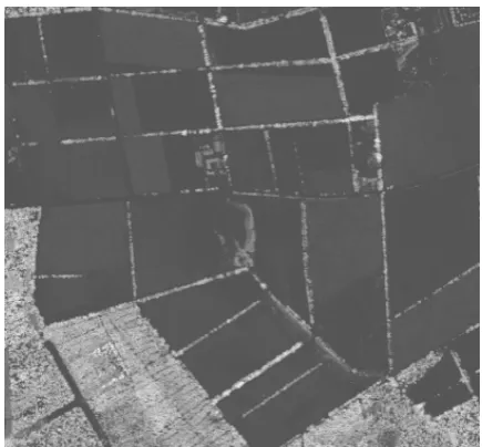
For our analysis, we obtained AISA Eagle data at about 800m altitude with 107 spectral bands in the range between 431 and 926nm and a spatial resolution of 0.5m. The spectral resolution in our data set was between 4.27 and 4.81nm. The single strips have been pre-processed be the data provider to form an image mosaic. Sample data can be seen in Figure 2. Due to turbulences while acquiring the data sets, the resulting data shows small artefacts such as straight lines being represented in wavy.
Figure 2. Central infrared bands of AISA Eagle acquired above our test site in western Germany. The scene comprises agriculture as well as forests and small settlements. Note the
wavy roads, especially in the top left, which are a result of additional movement of the aircraft during image acquisition.
This data set will be replaced with freely available Sentinel-2 data. For the purpose of this study, however, we artificially coarsen the spectral resolution to match that of Sentinel-2 (see section 4.2).
3.3 LIDAR
For our test scenario, LIDAR data was acquired synchronously to the hyperspectral information using a RIEGL LMS-Q680i full waveform laser scanner. The information is delivered in binary LAS file format. This format is used to exchange 3-dimensional data clouds and supports up to 15 return pulses from a target (ASPRS, 2011). This high echo rate is important for vegetation as different height layers of intertwined leaves and branches of the vegetation return multiple pulses. An analysis of these pulses results in a good knowledge of the type of vegetation. Figure 3 shows sample data of the LIDAR acquisitions at the same location in space and time as Figure 2.
Figure 3. Example data from the LIDAR acquisition. This scene represents the same temporal and spatial location as depicted in Figure 2. Higher structures (mainly vegetation but
also some houses) have lighter shades of grey.
An alternative to such LIDAR scenes is the estimation of height information using aerial photos for stereo matching. We will also focus on this alternative for future biomass mapping.
3.4 GIS
After having detected and quantified the vegetation using the combination of data sources described above, we compare the results to GIS maps which show road networks and communities in addition to transportation restrictions like height clearances, restrictions on highways or within cities or villages. A detailed analysis of the ideal collection spot as well as transport route and destination is possible. We can define spatial areas which serve a specific community or vary those over the years as different harvests become available. A detailed description of these steps is not part of this paper but will be done in the follow-up study.
4. METHODS 4.1 Vegetation height map
As the LIDAR data consists of a point cloud with up to 15 return pulses, a classification between non-ground points (i.e. vegetation) and ground (i.e. terrain) points is applied. For the purposes of LIDAR, anthropological structures like houses are classified as ‘terrain’ features as the only returning pulse will be from the surface as opposed to the leaf-branch structure in vegetation which returns multiple pulses. Out of these multiple pulses, the first is taken to represent the surface of the vegetation and the final characterises the ground. The vegetation height is determined by the difference between the first and last pulse. Soil and sealed surfaces (e.g. buildings and roads) have only one return pulse and their height is set to zero.
To assign the vegetation height to each pixel in our data set, we need a regular interval of LIDAR data points. We achieve this by using all available, irregularly distributed, LIDAR points to span a triangulated irregular network (TIN). A linear interpolation between the knots of this raster will yield the height data for all pixels. Since the LIDAR point cloud used at our test site was acquired synchronously to the spectral information, its density is very high. The resulting interpolation errors of this method are, therefore, negligible.
4.2 Sentinel-2 simulation
The Sentinel series is part of the Copernicus Programme of the European Commission. Sentinel-1, equipped with C-Band synthetic aperture radar (SAR) was launched in April 2014 with Sentinel-2 scheduled to follow in 2015 (Drusch et al., 2012). As opposed to Sentinel-1, the Sentinel-2 data stream will be recorded in the visible, near infrared and shortwave infrared over 13 spectral bands: four bands at 10m, six bands at 20m and 3 bands at 60m spatial resolution. The Swath width will be 290km. The temporal resolution is planned to be about five days, making use of the two scheduled satellites.
Since the AISA Eagle data set has a fine spectral resolution, we use that data set to simulate Sentinel-2 data the way we expect them to look in the identical settings. We use a simplified method for the generation of this data set as opposed to more complex sensor models described by Segl et al. (2012).
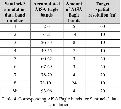
Initially, we determined the corresponding bands between AISA Eagle and Sentinel-2. As both systems are hyperspectrally recording, there is a certain similarity allowing us to correlate the data. As an example, Sentinel-2 band 1 data is spectrally located between 433 and 453nm. The same range also holds five AISA Eagle bands (bands 2 to 6), which will form the basis for Sentinel-2 band 1 data generation. The complete correlation between bands is shown in Table 1.
Following up on this correlation, the digital numbers (DN) of the Sentinel-2 pixels are calculated by averaging the DN values of all respective AISA Eagle bands according to Equation 1, where ti is the band number of Sentinel-2, sn the band number
of the AISA Eagle dataset and n is the total number of AISA Eagle bands needed to simulate the given Sentinel-2 band.
Sentinel-2
Table 4. Corresponding AISA Eagle bands for Sentinel-2 data simulation.
Finally, all DN values are normalised between 0 and 1 and resampled so that the spatial resolution of the Sentinel-2 data is achieved. An example RGB comprising Sentinel-2 simulated bands 2 to 4 with a spatial resolution of 10m created by using AISA Eagle bands between 8 and 55 can be seen in Figure 5.
Figure 5. Simulated RGB data set representing the Sentinel-2 bands 2 to 4. The scene is spatially and temporally identical to
Figures 2 and 3. The spatial resolution here is 10m.
4.3 Spectral unmixing
With the limited spatial resolution of the Sentinel-2 data, the pixel values will be comprised of a range of spectral signatures belonging to different features on the ground. A classification based on this data alone is limited. Our target vegetation has a width down under 5m for individual specimen and, thus, will not be detectable in larger pixels due to the mixture of different spectral signatures. We performed a spectral unmixing approach to find the endmembers in each pixel
(1)
which allows us to identify specific vegetation types and, in turn, their relevant biomass.
Regular classifications - supervised and unsupervised - assign only one class, the most probable, to each pixel. Spectral unmixing, on the other hand, treats each pixel as a mixed spectrum and decomposes it into different constituent spectra, the endmembers. Each endmember is associated with an abundance, the fraction it takes of the pixel. The endmembers represent pure reflectances for each surface (i.e. a specific vegetation type, a road, water, soil etc.). The spectral unmixing is a two-step approach: The endmember detection and the unmixing of the mixed reflectance.
In our study, we use the Sequential Maximum Angle Convex Cone (SMACC) approach introduced by Gruninger et al. (2004). It is available in the software ENVI and works with a convex cone, generated by using extreme vectors of the data (i.e. endmembers). The SMACC method works unsupervised. Initially, SMACC considers the pixel as pure and only assigns one endmember. After several sequences, this number is increased to incorporate more endmembers and, as such, more dimensions in the convex cone. The cone itself encompasses all vectors, i.e. mixed pixels, which can be created by the pure endmembers. The more endmembers are identified, the smaller the maximum relative error (MRE) becomes. The algorithm ends when either the maximum number of endmembers is reached or the MRE drops below a given percentage. An example of the relationship between found endmembers and MRE is given in Figure 6. With a very low number of endmembers, the maximum relative error is almost at 1, whereas it drops considerable fast once the next two endmembers are found. At a rate of four identified endmembers, the MRE reached a level of below 0.1 from where it only slowly converges on 0.
Figure 6. SMACC output showing the relationship between the number of identified endmembers and the maximum relative
error (MRE). The SMACC algorithm ends when either the MRE drops below a given threshold or a certain number of
endmembers are found.
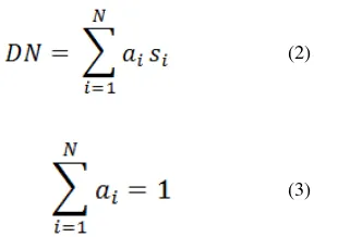
As the second step, a linear spectral unmixing (LSU) is applied. This part of the algorithm involves a linear mixture model detailed in Equation 2, where DN is the digital number of each pixel, N represents the number of endmembers, ai the
abundance of endmember i and si the spectrum of endmember
i. The sum of all abundances ai have to add up to 1 (Equation
3).
The outputs of this analysis are the individual, extracted endmember spectra (Figure 7) along with their abundances. In addition, separate endmember locations within the imagery are yielded which allow for the analysis of biomass concentrations.
Figure 7. Example of found endmember spectra over the first four bands of the Sentinel-2 data. The spectra represent normalised pixel values (NPV). It can be seen that some are
more similar than others.
4.4 Potential map
As the ultimate step in this initial phase of the project, a biomass availability (or biomass potential) map is created. This map will have multiple layers of information to identify the biomass and its feasibility to be used as renewable energy. The basis for this map is the spectral unmixing of the Sentinel-2 data (initially, the simulated and, later, the official data sets) as well as the DSM. Additionally, GIS data sets like a road networks, preferred biomass accumulation areas and transport limitations are incorporated. Other GIS objects like rivers and railways can also function as proxies as to where biomass is available.
The spectral unmixing based on the SMACC method is unsupervised. Due to this, the resulting abundance maps need to be manually verified regarding the objects of interest represented by them. Two examples are in Figures 8 and 9. Figure 8 shows the abundance map of endmember 4, which represents vegetation in general, whereas endmember 8 (Figure 9) only corresponds to vegetation to agricultural crops. The whiter the pixel in those Figures, the higher is the abundance of the respective endmember.
Number of Endmembers MRE
1 2 3 4 Band Number
NPV
(2)
(3)
Figure 8. Endmember 4 abundance map. The brighter the pixel, the higher is the percentage of the fourth endmember
(general vegetation) in the image.
Figure 9. Endmember 8 abundance map. The brighter the pixel, the higher is the percentage of the eighth endmember
(agricultural crops) in the image.
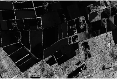
The LIDAR-based DSM is considered to be a direct indicator for biomass (Figure 10). The whiter a pixel in this the DSM, the higher the corresponding structure is. Artificial structures like houses have been removed in the due to their single-pulse nature.
Figure 10. LIDAR-derived DSM showing all vegetation as grey pixels whose brightness increases with height above ground.
5. DISCUSSION AND CONCLUSIONS
This proposed methodology is applied to test data from a site in Germany, close to the city of Bottrop in North Rhine-Westphalia. The test site is located in a rural area with intensive agricultural use but contains also parts of a natural preserve, including forests, as well as some settlements.
To evaluate our method, we chose to create a vegetation abundance map solely using spectral unmixing as described above, i.e. without the height information (Figure 11). This map can then be compared to a vegetation reference map based on LIDAR data (Figure 12). Both maps are binary. The vegetation map combines all abundance maps where each pixel is set to 1 when one or more endmembers are determined to resemble more than 50% of the pixel. It thus shows the area that is identified as vegetation using only spectral information. The reference map also shows vegetation higher than 0.3m but, in this case, the information directly comes from LIDAR data. A matching vegetation outline thus shows a good assessment with the two chosen methods and a good data correlation for height determination.
Figure 11. Vegetation map created solely based on unmixing of the spectral data sets without additional information from the
DSM. All green pixels represent vegetation.
Figure 12. Vegetation reference map solely obtained through LIDAR data. All green pixels represent vegetation higher than
0.3m.
A pixel-to-pixel comparison between both maps shows a vegetation match of 74.5%. When calculating the accuracy of the vegetation map alone (Figure 11), 69.8% of all biomass in the map is also classified as such in the reference whereas 30.2% are misclassified. Errors can be introduced due to the 0.3m minimum height required for the reference map as well as a wrong amount of endmembers taken during the SMACC calculations.
Evaluations of single biomass entities prove difficult as the reference data is rare. However, the vegetation height map (Figure 10) shows a great amount of detail and, when combined with other data sources to the biomass potential map, will prove very valuable in detecting small scale features.
The aim of the approach presented here is the mapping of previously largely ignored biomass sources important for energy production. To keep the data costs at a minimum, we aim to use the upcoming Sentinel-2 data sets, which will be freely available. In addition, we use height information based on LIDAR and, where available, aerial imagery..
The results of our study here are the creation of information layers, which can then be built upon to subsequent biomass quantifications. In combination with GIS data, the results will prove valuable in outlining biomass rich areas as well as logistically important places and times for pick-up and transport of the harvested vegetation.
ACKNOWLEDGEMENTS
The research is done within the joint research project BiomassMon (Phase 2) (http://www.biomassmon.info/) that is funded by the Federal Ministry of Economics and Technology (BMWi) via the German Aerospace Center (DLR e.V.) under the funding numbers 50EE1333, 50EE1334 and 50EE1335.
REFERENCES
Ahamed, T., Tian, L., Zhang, Y., Ting, K.C., 2011. A review of remote sensing methods for biomass feedstock production. Biomass and Bioenergy, 35(7), pp. 2455–2469.
ASPRS, 2011. LAS 1.4 Format Specification. http://www.asprs.org/a/society/committees/standards/LAS_1_4 _r13.pdf (14 Nov. 2011)
Bargiel, D., 2013. Capabilities of high resolution satellite radar for the detection of semi-natural habitat structures and grasslands in agricultural landscapes. Ecological Informatics, 13, pp. 9–16.
Drusch, M., Del Bello, U., Carlier, S., Colin, O., Fernandez, V. Gascon, F., Hoersch, B., Isola, C., Laberinti, P., Martimort, P., Meygret, A., Spoto, F., Sy, O., Marchese, F., Bargellini, P., 2012. Sentinel-2: ESA's Optical High-Resolution Mission for GMES Operational Services. Remote Sensing of Environment, 120, pp. 25-36.
Estornell, J., Ruiz, L. A., Velázquez-Martí, B., Hermosilla, T., 2012. Estimation of biomass and volume of shrub vegetation using LiDAR and spectral data in a Mediterranean environment. Biomass and Bioenergy, 46, pp. 710-721.
Field, C. B., Lobell, D. B., Peters, H. A., Chiariello, N. R., 2007. Feedbacks of Terrestrial Ecosystems to Climate Change. Annual Review of Environment and Resources, 32, pp. 1-29.
Forzieri, G., 2012. Satellite retrieval of woody biomass for energetic reuse of riparian vegetation. Biomass and Bioenergy, 36, pp. 432-438.
Hepbasli, A., 2008. A key review on exergetic analysis and assessment of renewable energy resources for a sustainable future. Renewable and Sustainable Energy Review, 12, pp. 593-661.
Gruninger, J. H., Ratkowski, A. J., Hoke, M. L. 2004. The sequential maximum angle convex cone (SMACC) endmember model. SPIE Proceeding, Algorithms and Technologies for Multispectral, Hyperspectral, and Ultraspectral Imagery, 5425 (1), doi:10.1117/12.543794.
Popescu, S. C., 2007. Estimating biomass of individual pine trees using airborne lidar. Biomass and Bioenergy, 31 (9), pp. 646-655.
Segl, K., Guanter, L., Rogass, C., Kuester, T., Roessner, S., Kaufmann, H., Sang, B., Mogulsky, V., Hofer, S., 2012. EeteS—The EnMAP End-to-End Simulation Tool. IEEE Journal of Selected Topics in Applied Earth Observations and Remote Sensing, 5(2), pp. 522-530.
Specim, 2014. Aisa EAGLE Hyperspectral Sensor. http://www.specim.fi/files/pdf/aisa/datasheets/AisaEAGLE_dat asheet_ver1-2013%281%29.pdf (29 Jun. 2014).
Voivontas, D, Assimacopoulos, D, Koukios, E. G., 2001. Assessment of a biomass potential for power production: a GIS based method. Biomass and Bioenergy, 20, pp. 101-112.