222
The Impact of Financial Ratio toward Stock Return of Property Industry in
Indonesia
Kevin Stefano
International Business Management Program, Petra Christian University Jl. Siwalankerto 121-131, Surabaya
E-mail: [email protected]
ABSTRACT
Indonesia property industry is one of the most booming sectors in recent years. The growth of property companies’ stock return is higher than overall stock index after β009. This research is conducted to identify whether financial ratio, as a representative of companies financial performance, has significant impact toward the booming stock return of property industry. The data was gathered using judgement sampling by generating the financial ratio of 18 property companies listed in Indonesia Stock Exchange. The data was analyzed by using Multiple Linear Regression Analysis. The result shows that financial ratio simultaneously have significant impact toward the stock return. Meanwhile, i n d i v i d u a l l y , only Return on Asset has the significant impact toward stock return of property industry in Indonesia.
.
Keywords: Financial Ratio, Stock Return, Property Industry, Indonesia
ABSTRAK
Industri properti Indonesia adalah salah satu sektor yang paling populer dalam beberapa tahun terakhir . Setelah tahun 2009, pertumbuhan return saham perusahaan properti lebih tinggi dari Indeks Harga Saham Gabungan. Penelitian ini dilakukan untuk mengetahui apakah rasio keuangan, sebagai bukti dari kinerja keuangan perusahaan , memiliki dampak yang signifikan terhadap return saham perusahaan dari industri properti. Metode pengumpulan data menggunakan judgment sampling dengan data rasio keuangan 18 perusahaan properti yang terdaftar di Bursa Efek Indonesia. Data dianalisis dengan menggunakan Analisis Regresi Linear Berganda. Hasil penelitian menunjukkan bahwa rasio keuangan secara simultan berpengaruh signifikan terhadap return saham. Sementara itu, secara individu, hanya Return on Asset memiliki dampak yang signifikan terhadap return saham industri properti di Indonesia
.
Kata Kunci: Rasio Keuangan, Return Saham, Industri Properti, Indonesia
INTRODUCTION
Indonesia property sector is one of the most noticeable sectors recently. How it performed in the era of post financial tsunami worth noticing. In 2009, the effect of financial crisis severely hit the property industry in Indonesia resulting in slowdown of property companies’ stock return. Global financial crisis reduced the listed property companies’ performance in Indonesia by 55% (Newell & Razali, 2009). In 2009, property index grew by around 38.35% along the year. However, property index growth was below the average of Indonesia’s stock market by the difference of around 7.78%. Surprisingly, a huge resurgence occurred in 2010 where property index grew almost 10% above the average of IHSG. This is quite a startling jump considering that the index grew below the
223
year on year, while in 2011, it rose by 4.54% year on year (Bank Indonesia, 2009-2013)..The escalation of property price was accompanied with another phenomenon regarding banking credit. On average, credit rate given by most banks is getting lower since 2009 (Suku Bunga Kredit Rupiah Menurut Kelompok Bank, 2014). A survey conducted by Direktorat Statistik Moneter (DSM) and Direktorat Penelitian dan Pengaturan Perbankan (DPNP) of Bank Indonesia in 2012 shows that historically there is a correlation between rise in property price and growth in property credit. Bank Indonesia also stated that one of the causes for growth in property credit is interest rate (Tim Statistik Sektor Riil Bank Indonesia, 2011). As a matter of fact, property credit, consisting of Housing Credit (KPR) and Apartment Ownership Credit (KPA), had contributed the biggest growth for consumption credit in Indonesia during 2011 (Bank Indonesia, 2011). Thus, rise in property price and lower interest rate is the main reason of significant growth of property credit. Based on the situation and condition of property that already described, it is interesting to examine the impact of property companies’ financial performance, influenced by the condition above, toward their stock return. By finding out the answer, research will be able to reveal whether the resurgence of property index post financial crisis is influenced by the companies’ financial performance, measured by its financial ratio.
This research will discuss the problem whether profitability ratio, liquidity ratio, debt ratio, market ratio, and activity ratio simultaneously and individually have significant influence toward stock return of Indonesia property industry. Hypothesis testing will be conducted to test whether profitability ratio, liquidity ratio, debt ratio, market ratio, and activity ratio simultaneously and individually have significant influence toward stock return of Indonesia property industry.
LITERATURE REVIEW
In understanding the topic and flow of the research, researchers must first identify and explain the theory that will be the foundation of this research. The first theory will be discussed is surely about financial ratio and the components within. Another theory that researchers is about to use is regarding stock return. The expanded explanation of these theories will be discussed in the following part of the research..
Concept of Financial Ratio
According to Bambang Riyanto (2001), financial ratio is the measurement used by a firm to analyze and interpret its financial position. Another definition by Horne & Wachowicz (β007) saying that financial ratio is “an index which relate two accounting numbers and the result is obtained by dividing one particular number to the other”. The data source of financial ratio is coming from financial statements produced by companies every year. Basically, there are two methods can be used in analyzing financial ratio: cross sectional and time series analysis. Cross
sectional analysis focusses in comparing the financial ratio of firms at the same point of time. It tries to make a comparison of a firm’s ratios to the average of the industry. Another method in cross sectional analysis is benchmarking where a company’s financial ratio is being compared to key competitors that it expects to contend with (Gitman & Zutter, 2012)
Another method for computing financial ratio is time series analysis, where it is used to evaluate financial performance of a company over time. The factor being compared is current to past performance that will enable analyst, investors, and shareholder to track the firm’s progress. (Gitman & Zutter, 2012). For convenience, Gitman & Zutter (2012) divided financial ratio into five basic categories: profitability ratio, liquidity ratio, debt ratio, activity ratio, and market ratio. Previous researches conducted by various researchers use one representative ratio for each financial ratio. Savitri (2003) used current ratio and debt to equity ratio (DER) as representatives for liquidity ratio and debt ratio respectively. Another research by Ika (2013) used total asset turnover, return on asset, and price earning ratio as representatives of activity ratio, profitability ratio, and market ratio respectively. Therefore, this research will also take one equation in each ratio that will be tested to the dependent variable. Detailed explanation about each of the ratio and equation is as follows:
1. Profitability ratio is used to evaluate a firm’s profit given its number of assets and owner’s investment. Researcher will use ROA to represent this ratio as have been used by previous research of Ika (2013). The formula to calculate ROA is to divide the Earnings available for common stockholders by the Total Asset.
2. Gitman & Zutter (2012) states that liquidity ratio measures the firm’s “ability to satisfy its short term obligation as it comes due” (p. 71). One of the measurer of liquidity ratio that researcher will use is current ratio. It is also confirmed by the research from Kusumo (2011) which also used current ratio to gauge liquidity ratio. Current ratio will reveal the capability of a firm to repay its short term debt. The formula to calculate current ratio is dividing Current Asset by Current Liabilities.
3. Debt ratio is “the amount of other people’s money being used to generate profits” (p. 76). The debt ratio used in this research is debt to equity ratio (DER), which will calculate the percentage of total assets financed by creditors (Weygandt, Kimmel, & Kieso, 2010). The formula to calculate debt ratio is total liabilities over total shareholder’s equity.
4. Generally, this ratio is a measurement of the efficiency of a firm considering its asset, disbursement, collection of receivables, and inventory. Total asset turnover will be the activity ratio used by researcher. It indicates how efficient a firm can generate sales by in regards to the use of its asset. The more efficient the firm, the higher the asset turnover is. Sales and total assets will be the determinants to calculate total asset turnover (Gitman & Zutter, 2012).
224
This ratio can give an indication of how the performance of firm, in term of risk and return, is perceived by investors (Gitman & Zutter, 2012). The most common market ratio is P/E ratio, which “assess the owner’s appraisal of share value” (Gitman & Zutter, β01β, p. 8β). The indicators of P/E ratio consist of market price per share of common stock and earning per share (EPS). Market price per share of common stock is the price that investors must pay to acquire one share of a company’s common stock (Gitman & Zutter, β01β, p. β68), while EPS is “a measure of the net income earned for each share of common stock”.Concept of Stock Return
Stock return is defined as the capital gain or loss of as a result of investing in stock portfolio (Jones, 2000). The concept of selecting stock portfolio must be started with theory of Markowitz Portfolio Selection (1952). Investors must always aim at maximizing expected return of their portfolio, subject to acceptable level of risk. Markowitz (1952) stated that the more stocks added to the portfolio of investors, the risk will be higher, represented by its standard deviation. Investors though, will always seek to maximize its return by staying within the efficient frontier in regards to standard deviation
Following the theory of portfolio selection by Markowitz (1952), investors are assumed to be rational. Rational means that they react quickly and objectively to new information in order to seek for the best profit of their investment (Gitman & Zutter, 2012). This will lead to a theory called Efficient Market Hypothesis developed by Eugene Fama in 1960s, where it explains the trait of a “perfectly efficient” market. However, not all investors follow the idea of Efficient Market Hypothesis that was originated by Eugene Fama (1960). Gitman & Zutter (2012) states that some investors feel it is worthwhile to find overvalued and undervalued stocks price and earn profit from the market inefficiencies. In summary, this behavior of investors that often attempt to find mispriced stocks leads to capital loss or gain by investors themselves. This explains the existence of stock return in the market as researchers firstly define stock return as the gain or loss of investment (Jones, 2000). Referring to Jogiyanto (2000), the formula used to calculate the stock return of investors is as follows: Rt = Pt – P(t-1) / P(t-1)
Relationship between concepts
The theories developed for this research consist of theory of financial ratio and theory of stock return. Financial ratio shows the overall evaluation of firm financial performance and position (Riyanto, 2001), while stock return is a measurement of capital gain or loss as a result in investment in stock securities (Jones, 2000)
The financial ratios being used are profitability ratio, debt ratio, liquidity ratio, activity ratio, and market ratio. The figure to explain the relationship between variables is as follows:
Figure 1. Relationship Between Concept
As the fundamentals of the research, researchers have developed two hypotheses to predict the outcome of the research. The hypotheses are as follows:
H1: Profitability ratio, liquidity ratio, debt ratio, market ratio, and activity ratio simultaneously has significant impact toward stock return on Indonesia property industry
H2: Profitability ratio, liquidity ratio, debt ratio, market ratio, and activity ratio individually have significant influence toward stock return on Indonesia property industry
The backgrounds why researchers come up with these hypotheses have been shown from the previous researches conducted by various researchers. In most of the researches, the authors always start assuming that all ratios should have significant influence toward stock return. It is also in line with the explanation that financial ratio commonly used by investors to evaluate the performance of a firm before finally deciding to buy its stocks (Gitman & Zutter, 2012).
RESEARCH METHOD
Since the purpose of this study is to explain the impact of financial ratio toward stock return, then it is reasonable to classify this study as explanatory study. It is also justified to state that the appropriate approach used in this research is quantitative research since the researchers wanted to test and verify previous theories having been conducted by other researchers. The result of this research will be able to test and confirm the theories and hypothesis developed pre research. The data gathered in this research will be analyzed using SPSS v.20 and multiple regression analysis as the statistical tool..
225
calculation is taken from the financial statements published by the listed property companies to Indonesia Stock Exchange. On the other hand, the data for stock return will be taken from historical price of stock published in Indonesia Stock Exchange. Another sources of secondary data used in this research are articles, journals, report, and books.The sampling method used in this research is nonprobability sampling since researchers will subjectively choose the sample that fulfill certain criteria. The classification of sampling method is judgement sampling as researchers will define several relevant characteristics then determines number of samples based on the biggest market capitalization to represent the population. In this case, researchers need to find sample that is reliable to represent the population of all listed property companies in IDX, amounted up to 46 (Exchange, Fact Book , 2014). The time frame of this research will be from 2009-2013. . In order to ensure the availability and accessibility of data, researchers will set two criterias. Firstly, all companies must have its IPO before 2009. Next, all companies’ financial statement must consistently be published in Indonesia Stock Exchange during 2009-2013.
After setting the criteria, researchers will then attempt to determine the minimum sample size. In order to determine the number of sample that will be used for the research, researcher will be using the theory developed by Hair, Black, Babin, & Anderson (2010). They stated that “larger sample sizes reduce the detrimental effects of non -normality” (p. 71). In sample of less than 50 observations, the variation from normality will significantly impact the result of the research. Therefore, in this case, researcher decides to take the sample of 90 observations to fulfill the criteria of minimum 50 observations. Researcher will choose 18 companies and use the data from all those companies for period 2009-2013. Then, the total number of sample will be exactly 90 samples. The justification of choosing 18 companies will be based on the highest market capitalization. The reason why researcher uses market capitalization to determine the companies that represent property industry is because market capitalization is also used as the base calculation of to calculate sectorial index, in this case property index (IDX, 2010)
As previously mentioned above, researcher draws the data for this research only from secondary sources. The method to find data about financial ratio and stock return are as follows:
1. Documentation of financial ratio, by collecting, calculating, and analyzing the secondary data from the financial statement of property companies registered in Indonesia Stock Exchange during 2009-2013 as listed in the latest Fact Book 2014 of Indonesia Stock Exchange.
2. Documentation of stock return, by collecting the data of historical closing price of property companies stock as provided by Indonesia Stock Exchange during 2009-2013.
According to Standar Akuntansi Keuangan (2002), financial statement is normally used by related parties like investors, creditors, employees, customers, and even
government to fulfill their different requirement of company’s information. while Indonesia Stock Exchange (IDX) is the official market platform that comprises the trading process of various market instruments such as stock, bonds, derivative, and mutual fund (Exchange, IHSG, 2010). The usage of sources from Indonesia Stock Exchange as official platform of market trading and company’s financial statement as the measurement of companies’ performance will ensure the validity and reliability of the data used in this research.
The statistical process of this research will mainly be divided into two main parts; classical assumption test and multiple linear regressions. Researchers will firstly process the data into classical assumption to make sure the quality of the data. Then, the data will be further analyzed using multiple linear regression to interpret the result and draw conclusion of the data. There will be 4 type of classical assumption test conducted by researcher this time; normality test, multicollinearity test, heterocedasticity test, and autocorrelation test. All the information about classical assumption test will be based on Ghozali (2006);
According to Ghozali (2006), normality test purposes to test whether the residual variable in the regression model is normally distributed. The ideal residual value should follow the normal distribution, otherwise it would be considered as an invalid statistical test. There are two methods in doing the normality test, graphical analysis and statistical analysis. Graphical analysis is a statistical test of residual plot by observing model in the form of histogram and normal plot. Another method is to observe the normal probability plot and compare the cumulative distribution and normal distribution. Typically, normal distribution will be in the form of one diagonal line and the residual data plot should scatter consistently following the diagonal line.
Another form of normality test is statistical test. The statistical analysis can be conducted by seeing the kurtosis and skewness value of residual. Z statistic for skewness can be calculated as follows: Z skewness = Skewness/(√6/N). While the value of Z kurtosis is as follows:
Z Kurtosis = Kurtosis / (√β4/N).
Multicollinearity test aims to test whether a correlation between independent variables exist within the regression model. Valid regression model should not contain correlation among independent variables (Ghozali, 2006). In this research, the method used to detect the existence of multicollinearity is by seeing the value of tolerance and Variance Inflation Factor (VIF) in the regression model. These two factors show which independent variable is explained by other independent variables. High correlation between independent variable means that an independent variable acts as dependent variable toward the other independent variable. Value of tolerance ≤ 0.10 or VIF ≥ 10 indicates the existence of multicollinearity.
226
potentially influence the problem to that similar data for the next period. Good regression model shall be free from autocorrelation indication. The method to detect autocorrelation in this research will be Durbin Watson test. The null hypothesis for Durbin Watson test stated that there is no autocorrelation on residual data, while alternate hypothesis state otherwise.Ghozali (2006) stated that heteroscedasticity test has the main goal to detect the difference of residual variance between observations or collected data. If there is no difference on residual variance, then the data is considered as having homocedasticity. Valid data should represent homocedasticity, meaning that there is no different on residual variance between observed data. The method in used in this research to detect the existence of heteroscedasticity is Glejser test, which will conduct regression of the absolute residual value toward independent variable (Ghozali, 2006)
The next statistical process conducted in this research is multiple linear regression. According to Pallant (2005), multiple linear regression “explore the relationship between one continuous dependent variable and a number of independent variables or predictors” (p. 140). Multiple linear regression can indicate the strength of relationship as well as the positive or negative value of dependent and independent variable. Based on (Cooper & Schindler, 2014, p. 477), the equation for multiple linear regression is as follows:
=α+ b1x1+ b2x2+ b3x3+...+ b5X5 Another subject of multiple linear regression is hypothesis testing. Hypothesis testing can be conducted simultaneously, with F test, and individually, with t-test. According to Ghozali (2006), F test will show whether all independent variable simultaneously impacting the dependent variable. The interpretation of this F test can be done in two ways. First, Ho is rejected when the F value is larger than four with five percent significance level. This research will use the alpha or significance level of five percent. If the value of significance probability in SPSS is smaller than the alpha (five percent), then alternate hypothesis shall be accepted. Another way to interpret the result is looking at the F value in SPSS calculation and compares it with F according to table. When F value in SPSS is larger than F table, Ho should be rejected and accept H1 instead.
On the other hand, t-test will try to test whether independent variable individually impacting the dependent variable (Ghozali, 2006). Based on Ghozali (2006), the interpretation of result of t-test can be done by observing the significance of the independent variable and compare it to the designated alpha, which is five percent. If the t-significance (p value) is lower than 0.05, then Ho is rejected and accept the alternate hypothesis. Another method is to see the t-value and compare it to the t critical value from the table. If t value (t-test statistic) from SPSS computation is higher than t-table, then Ho should be rejected. The Constanta appeared on the unstandardized coefficient will also serves as measurement of the sensitivity of the
dependent variable toward the change in independent variable.
According to Ghozali (2006), R2 will be one factor appear on multiple linear regression analysis. It basically measures the extent to which the independent variables can explain the dependent variable. Small value of R2 indicates the very limited ability of independent variable to explain the dependent variable. The weakness of R2 is the bias due to the number of independent variable added into the equation. As one independent variable added, R2 tends to get larger regardless the significant impact of the added variable. Therefore, it is recommended to use adjusted R2, whose value might rise or fall according to the significant impact of the added variable (Ghozali, 2006). Thus, researcher will use adjusted R2 to assess the ability of independent variables to explain the dependent variable
RESULTS AND DISCUSSION
Before conducting analysis on the data, researchers will have to do classical assumption test on the collected sample. There are four types of classical assumption done in this test; multicollinearity test, heteroscedasticity test, autocorrelation test, and normality test. Before passing the entire classical assumption test, researchers have attempted to test all the 90 variables yet failed to pass heteroscedasticity and normality test. Since the original data of 90 sampling do not pass the entire assumption test, then researcher decided to remove outliers by deleting them per data sets (Ghozali, 2006). The reason why researcher use this method is due to the problem in heteroscedasticity of independent variable of PER. There are some PER data that have extreme value leading to the existence of some extreme residuals. Therefore, researcher decides to remove the outliers from the observation data. Since PER is the troubled set of data, researcher removes the outliers in PER using boxplot analysis in SPSS. Then, the outlier for the dependent variable of return is also removed using the same method of boxplot observation in SPSS. In total, there are 12 data sets considered outliers that have been removed by researcher. After removing the outliers, researcher found the data finally passed all the classical assumption.
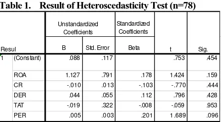
Table 1. Result of Heteroscedasticity Test (n=78)
Based on the result of the table above, all variables have significance value higher than 0.05. The lowest value of significance is PER, which is 0.096. It means that this test failed to reject Ho, meaning that there is no heteroscedasticity within the residuals of the model. It also
Standardized Coefficients B Std. Error Beta
(Constant) .088 .117 .753 .454 ROA 1.127 .791 .178 1.424 .159 CR -.010 .013 -.103 -.770 .444 DER .044 .055 .112 .796 .428 TAT -.019 .322 -.008 -.059 .953 PER .005 .003 .201 1.689 .096 1
Resul
Unstandardized Coefficients
227
means that the residuals are consistent across different independent variables.Table 2. Result of Multicollinearity Test (n=78)
In this test, data is considered free from multicollinearity. Looking at the table above, each independent variable has the value of tolerance far above 0.1 with 0.640 as the lowest value. The VIFs are all also way lower than 10, with 1.563 as the highest value. It shows that there is no correlation between independent variable in this research. Therefore, data collected for sample are free from multicollinearity.
Table 3. Model Summary
The result of multicollinearity test can be observed from the table above. The Durbin Watson of the test is 1.851. The value of du and dl based on Durbin Watson table by Savin & White (1997), is 1.776 and 1.542 respectively. Therefore, taking the last decision criteria, du (1.776) < d (1.851) < 4-du (2.224). The value of Durbin Watson is in between the du and 4-du. The result of such criteria is to accept Ho, meaning that there is no autocorrelation existed in this research.
Table 4. Skewness & Kurtosis (n=78)
Figure 2. Histogram (n=78)
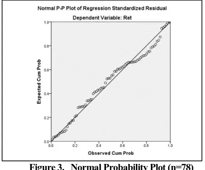
Figure 3. Normal Probability Plot (n=78)
Calculation of Z skewness and Z kurtosis is as follow: Z skewness = 0.020 /
The result of the data, whose outliers have been removed, shows the z skewness value 0.721 and z kurtosis 0.447. Both numbers are lower than z table 1.96, so the residual of data is considered normally distributed. Therefore, statistically it passes the normality test. Graphically, the distribution in histogram follows the normal distribution shape. The plot in normal probability plot also more consistently follows the diagonal line. It shows that this data finally passes the normality test both graphically and statistically.
The presentation of the result of multiple linear regression will be as follow:
Table 5. ANOVA Table
Based on the table above, the significance probability on SPSS is 0.002, smaller than the significance level or alpha. It means that simultaneously, the independent variables, financial ratios, have significant impact toward dependent variable, stock return. Another way to calculate is to compare the F value in SPSS statistic and table. Looking at the F table, researchers do interpolation to find the F value with df1 = 5 and df2 = 72.The result of F value of the data is 2.346, which is lower than the F computed on SPSS. It means the computed value of 4.248 falls in the rejection region, where Ho is rejected and H1 is accepted. Therefore, simultaneously, there are at least one independent variable has the ability to explain the variation in dependent variable.
The use of t test is to measure whether independent variable individually has significant impact toward dependent variable. The interpretation of result of t-test can be done by comparison between the significance level of the independent variable and the designated alpha, which in this case is five percent (Ghozali, 2006). Other method used
Tolerance VIF (Cons tant)
ROA .808 1.238
CR .707 1.414
DER .640 1.563
TAT .661 1.512
PER .890 1.123
Model
Collinearity Statis tics
1
1 .477a .228 .174 .3243721 1.851 Durbin-Watson Model R R Square
Adjusted R Square
Std. Error of the Estimate
N
Statistic Statistic Std. Error Statistic Std. Error Unstandardized
Residual
78 .020 .272 .248 .538 Valid N (listwise) 78
Skewness Kurtosis
Sum of Squares df
Mean
Square F Sig. Regression 2.235 5 .447 4.248 .002b
Residual 7.576 72 .105 Total 9.810 77 Model
228
is comparing the t-value of SPSS computation and t-value from the table with 0.05 significance level. The decision rule is that Ho failed to be rejected if significance level of t (p value) is higher than significance level (α) of 0.05 or if the t-value of SPSS between -1.991 (-t critical value) and 1.991 (+ t-critical value). However, if p value is lower than significance level (α) of 0.05 or t value of SPSS is either lower than -1.991 or higher than 1.991, then Ho is rejected, resulting to that particular variable is significantly impacting the dependent variable. The null and alternate hypothesis developed for each financial ratio is:H1: Return on asset has significant impact toward stock return ( = 1)
H2: Current ratio has significant impact toward stock return ( = 1)
H3: Debt to Equity ratio has significant impact toward stock return ( = 1)
H4: Total asset turnover has significant impact toward stock return ( = 1)
H5: Price Earning ratio has significant impact toward stock return ( = 1)
Table 6. Table of Regression Coefficient
= . + . − . + . −
. + .
The interpretation of result of the t-test conducted in this research per independent variable will be as follows: For Return on Asset, based on the table of regression coefficient above, the significance t of return on asset is 0.001 which is way lower than the significance level (α) of 0.05. The t value computed on SPSS, which is 3.534, is also a lot greater than 1.991. It means that the null hypothesis of return of asset is rejected and alternate hypothesis is accepted. Therefore, ROA individually has significant influence toward stock return. In addition, having the unstandardized coefficient of 4.451 indicates that for every 100% increase in ROA will elevate the stock return 4.451 times higher.
For current ratio, as the significance level of current ratio is 0.123, higher than alpha, and its F value is -1.559, higher than -1.991, therefore the null hypothesis is failed to be rejected. As a result, current ratio is considered insignificant factor of stock return in this research. Thus, although current ratio has the unstandardized coefficient of -0.033, it is inconclusive that for every 100% increase in current ratio, stock return will decrease as much as 3.3%, net of the effects of changes due to other independent variables.
Next, the result of DER is that the significance level of DER, 0.089, is higher than the alpha. While DER’s t value on SPSS of 1.721 is lower than 1.991. It means that the null hypothesis is failed to be rejected. Therefore, debt to equity ratio individually does not have significant impact toward stock return. Although, it has the unstandardized coefficient of 0.151 in regression equation, it cannot be concluded that for every 100% rise in DER, stock return will also raise 15.1%, net the changes of other independent variables.
As TAT’s significance level of 0.076 is higher than the 0.05 alpha and its tvalue of 1.803 is greater than -1.991, it is reasonable to conclude that Ho fails to be rejected. This result implies that total asset turnover is not a significant factor of financial ratio that influences stock return. Even though the coefficient of TAT in regression coefficient is -0.924, it does not conclude that for every 100% increase in asset turnover, stock return will fall as much as 92.4%, net the changes of other independent variables.
Based in the table of regression coefficient, the p value of PER is 0.093, greater than the alpha of 0.05. The t value is 1.705, lower than t table of 1.991. It means that null hypothesis failed to be rejected, and therefore alternate hypothesis is rejected. This means that PER does not have significant impact on stock return individually. So, PER’s coefficient of 0.008 cannot conclude that for every 100% increase in PER, stock return will also raise 0.8%, net the changes of other independent variables.
The next type of multiple linear regression anaylis is adjusted R Square. Adjusted R square is functioned to measures the extent to which the independent variables can explain the dependent variable, adjusted to the numbers of used independent variables. Looking at the table model summary 4.9, the adjusted R square for this research is 0.174. It means that only 17.4% of stock return on property industry can be explained by the financial ratio, accounted the sample size and independent variables
Below is the summary of the result of all independent variables:
Table 7. Summary of Result
*has significant impact toward dependent variable
Based on the table of summary of the result, only ROA the financial ratio which fulfill the decision criteria to reject Ho. The discussion of the result of each independent variable will be as follows:
Standardized Coefficients B
Std.
Error Beta
(Constant) .104 .186 .557 .579 ROA 4.451 1.259 .407 3.534 .001 CR -.033 .021 -.192 -1.559 .123 DER .151 .088 .223 1.721 .089 TAT -.924 .513 -.230 -1.803 .076 PER .008 .005 .187 1.705 .093 1
Model
Unstandardized Coefficients
t Sig.
Independent Variable
Unstandardized Coefficients
(Constant) .104
ROA* 4.451 3.534 .001
CR -.033 -1.559 .123
DER .151 1.721 .089
TAT -.924 -1.803 .076
PER .008 1.705 .093
229
It is found out that ROA individually has significant impact toward stock return. The significance of ROA means that the stock return of property industry is significantly determined by how much the asset can generate earning. It also implies that investors really value the ability of asset to earn profit in this particular property industry during the period. Looking at the summary of result, the significance of ROA is supported by previous research conducted by Ika (2013). In her research, which examined the impact of financial ratio toward stock return of food and beverage company in Indonesia, ROA was also stated as significant independent variable besides PER. It is stated that the main reason why ROA is significant is because investors believe that higher earning power is positively correlated to higher asset turnover or profit margin. The value of company is believed to be rising following the rise in ROA. This in turn will increase the stock return as perceived by investors (Ika, 2013). The significance of ROA is also justifiable because assets are financed from credit and equity, including equity from investors. When investors give credit in the form of shares bought, they must be concerned with how much the unit of assets, financed from their money, can give appropriate return to them. That is why the return of asset is an essential indicator that investors look closely to influence stock return (Saeidi & Okhli, 2012).Based on the t test result, current ratio individually does not have significant impact toward stock return on property industry. This result is consistent with the findings from Kusumo (2011) and Ika (2013). High current ratio might indicate that company has the ability to cover its short term debt, and therefore having enough current assets or liquid asset to be converted into cash. However, this might not be favorable in the eye of investors in the case of property industry since high current ratio can also mean companies have too much current assets (such as cash) on hand and might indicate difficulties in investing to other capital. (Kusumo, 2011). Current ratio can also be a mislead indicator of liquidity of a company in the eye of investors. Companies with high current ratio are not necessarily being able to cover its short term debt with its short term asset. This is because the component of current ratio includes other current asset, which is not cash, and it still does take time to convert all the current assets into cash to pay debt. Even companies with higher current ratio are not always considered more liquid if it needs more time to convert its other current asset (such as account receivable) into cash compared to companies with lower current ratio. Thus, the ability of company to convert its working capital asset into cash in order to cover its short term debt is the more relevant key to liquidity (Parrino, Kidwell, & Bates, 2012).
Based on the table above, the result of t test found out that DER partially does not have significant impact toward stock return in property industry. This result is consistent with three previous research conducted by Ika (2013), Kusumo (2011), and Ulupui (2007). The justification of the insignificance of DER is that DER can be a misleading indicator. Based on Khan & Jain (2007), there is not rigid rule to determine the ideal proportion of debt to equity. It
depends on the situation for particular case such as size of company, type of business, nature of industry, and degree of risk involved. For example, a company in a situation when income is stable is appropriate to have higher portion of debt compared to companies with fluctuated demand of products. A new company is more likely would tolerate the use of debt lower than the more established one. Companies in growth business cycle might decide to have more debt compared to companies which enter mature cycle. Therefore, it does make sense that the information of companies DER is not adequate for investors to estimate its stock return. The effectiveness of companies in turning the debt into profit is a more appropriate basis for investors to predict the stock return.
Total asset turnover is found out insignificantly impacting the stock return on property industry. This result is consistent with the findings from two previous researches of Ika (2013) and Ulupui (2007), while Kusumo (2011) stated otherwise. The reason why TAT is such insignificant factor for investors in estimating stock return is because TAT might give false expectation of profitability of a company. Companies with high TAT do not necessarily produce better return or higher profit. If the profit margin of companies is very low, then the high turnover of asset might lead to nothing. Thus, the risk of misperception surely leads to investors reluctant to use this ratio to predict stock return. PER is found to be insignificant on its impact toward stock return. This finding is not consistent with the research of Ika (2013), yet consistent with the findings from Savitri (2003). The reason why it is insignificant is because this ratio represents the result that investors enjoy and thus hardly used to predict the expected stock return of company (Savitri, 2003).
CONCLUSION
In Summary, the problem arises whether financial ratio has significant impact toward the stock return in property industry of Indonesia. Another question that was raised is which ratio has the most significant influence toward the stock return. In order to answers all those questions, researcher then construct two hypotheses. The first hypothesis tries to check whether financial ratio simultaneously have significant impact toward stock return of property industry in Indonesia, while the second hypothesis will test whether each financial ratio individually has significant impact toward stock return. To check the hypothesis, researcher then gathers the data from the samples of 18 property companies during 2009-2013. The data is derived from secondary source, which is from the report of Indonesia Stock Exchange as well as the financial ratio calculated from the financial statement of those companies. The data is then processed into classical assumption tests; normality test, multicollinearity test, heteroscedasticity test, and autocorrelation test. The result shows that the distribution of the data follows normal distribution and contains no autocorrelation, multicollinearity, and heteroscedasticity.
230
the first test conducted, which is F test, resulted in financial ratio simultaneously have significant impact toward stock return. The result of the t test verifies the second alternate hypothesis, with ROA as the only independent variable that significantly influences the stock return of property industry in Indonesia. Finally, it is conclusive that ROA has the biggest influence toward stock return since the coefficient in regression equation is higher than any other independent variables. However, it is also known that the adjusted R square is only 17.4%, which means that there is still 82.6% of the dependent variable cannot be explained by the independent variables.The conclusion and recommendation of this research have been made. Nevertheless, researcher realizes that there are still several limitations of this research. First, this research only uses independent variable which is derived from its internal performance, financial ratio. There are other external factors such as inflation, government policy, economic growth, interest rate that are not included in the coverage of research. Those external factors might also play important role in determining how the companies conduct business and eventually influence the output of this research. Further research can expand the area of coverage to the extent of external factors outside the companies.
Next, this research only uses five financial ratios as the independent variable to explain stock return of property companies. In fact, there are other financial ratios in the financial statement that is not covered in the research. Therefore, the recommendation given in this research is also limited to the coverage of how those five financial ratios could impact the stock return in property industry.
Considering the limitation mentioned above, there are some suggestions can be done by other researchers or academician to develop the topic. The first suggestion is to expand the area of coverage to the extent of outside company performance. Financial ratios, as the current independent variables, only consider internal companies’ performance as the factor influencing the stock return. However, there are many other external factors that influence the stock return in the eye of investors. Therefore, further research should be able to identify and include those other factors into the independent variable to better capture the predictability of stock return. Another suggestion is to add the independent variable within the internal performance of companies. As a matter of fact, the five financial ratios used in this research as independent variable have not covered all the financial ratios available in the financial statement. More independent variable of financial ratios can be included in further research to better explain the stock return of property companies in Indonesia.
REFERENCES
Andriansyah, Pohan, B., & Hosodo. (2007). On Free Float Shares Adjustment. Kertas Diskusi Bagian Riset Ekonomi, 2.
Bank Indonesia. (2009-2013). Survey Harga Properti Primer. Survey Report, Jakarta. Retrieved from http://www.bi.go.id/id/publikasi/survei/harga-
properti-primer/Documents/c3b16e074a0e4b6298aef2e8d39 6ce32shprtw4.pdf
Bank Indonesia. (2011). Survey Perbankan. Retrieved from http://www.bi.go.id/id/publikasi/survei/perbankan/D ocuments/3a12d8de7f5d4f5a830ad0fb1f533956skp tw4rev.pdf
Barber, B., & Odean, T. (2000). Trading Is Hazardous to Your Wealth: The Common Stock Investment Performance of Individual. Journal of Finance, 55, 773-806.
Berita Satu. (2012, March 19). BI: KPR dan KPA Tumbuh Tertinggi Dibanding Kredit Lain. Retrieved from http://www.beritasatu.com/ekonomi/37681-bi-kpr- dan-kpa-tumbuh-tertinggi-dibanding-kredit-lain.html
Brigham, E., Gapenski, L., & Ehmart, M. (1999). Financial Management Theory and Practice. Orlando: The Dryden Press.
Clarke, R. J. (2005). Research Models and Methodologies. HDR Seminar Series Faculty of Commerce Spring Session, (p. 7).
Cooper, D., & Schindler, P. (2014). Business Research Method (Vol. twelfth edition). New York: Mcgraw Hill.
Creswell, J. (2003). Research Design: qualitative, quantitative, and mixed methods approaches. Sage Publications, 18.
Direktorat Statistik Moneter, Direktorat Penelitian dan Pengaturan Perbankan. (2012). Survey Properti. Exchange, I. S. (2010). IHSG. Indeks.
Exchange, I. S. (2014). Fact Book . Jakarta.
Fama, E. (1970). Efficient capital markets: A review of theory and empirical work. Journal of Finance 25 (2), 383 - 417.
Ghozali, I. (2006). Aplikasi Analisis Multivariate Dengan Program SPSS. Semarang: Penerbit Universitas Diponegoro.
Gitman, L., & Zutter, C. (2012). Principles of Managerial Finance. Harlow: Pearson Education Limited. Hair, J., Black, W., Babin, B., & Anderson, R. (2010).
Multivariate Data Analysis. Pearson Prentice Hall. Horne, J. C., & Wachowicz, J. M. (2007). Fundamentals of
Financial Management: Prinsip-Prinsip Manajemen Keuangan (Vol. Edisi 12). (D. Fitriasri, & D. A. Kwary, Trans.) Jakarta: Salemba Empat. Retrieved March 4, 2015
IDX. (2010). Buku Panduan Indeks Harga Saham Bursa Efek Indonesia. Jakarta.
Ika, F. (2013). Pengaruh Rasio Keuangan terhadap Return Saham Perusahaan. Jurnal Unimus.
Indonesia Stock Exchange Research Division. (2012). IDX Statistics Book. Jakarta.
Indonesia, I. A. (2002). Standar Akutansi Keuangan. Jakarta: Salemba Empat.
Jogiyanto. (2000). Teori Portofolio dan Analisis Investasi. BPF-UGM.
231
Kahneman, D., & Tversky, A. (1979). Prospect Theory: AnAnalysis of Decisions under Risk. Econometrica, 47, 263-291.
Khan, M., & Jain, P. (2007 ). Financial Management. Mcgraw Hill.
Kusumo, G. I. (2011). Analisis Pengaruh Keuangan terhadap Return Saham pada Perusahaan Non-Bank LQ 45. Universitas Diponegoro.
Lulukiyah, M. (2011). Analisis Pengaruh Total Asset Turnover (Tato), Return On Asset (Roa), Current Ratio (Cr), Debt To Equity Ratio (Der) Dan Earning Per Share (Eps) Terhadap Return Saham. Journal Undip.
Maanen, J. V. (1979). Reclaiming Qualitative Methods for Organizational Research: A Preface (24 ed.). Administrative Science Quarterly 24.
Markowitz, H. (1952). Portfolio Selection. Journal of Finance, 77-91.
Newell, G., & Razali, M. N. (2009). The Impact of the Global Financial Crisis on Commercial Property Investment in Asia. Pacific Rim Property Research
Journal, 15. Retrieved from
http://www.prres.net/Papers/PRPRJ_No_4_2009_N ewell_Razali.pdf
Pallant, J. (2005). SPSS survival manual : a step by step guide to data analysis using SPSS. Sidney.
Parrino, R., Kidwell, D. S., & Bates, T. (2012). Fundamentals of Corporate Finance. WileyPlus. Puspitasari, F. (2012). Analisis Faktor-Faktor yang
Mempengaruhi Return Saham. Jurnal Universitas
Diponegoro. Retrieved from
http://eprints.undip.ac.id/35551/1/Skripsi_PUSPIT ASARI.pdf
Research Division of Indonesia Stock Exchange. (2009). IDX Statistics. Jakarta.
Riyanto, B. (2001). Dasar-Dasar Pembelanjaan Perusahaan (Vol. Edisi Keempat). Yogyakarta: BPFE UGM. Saeidi, P., & Okhli, A. (2012). Studying the effect of assets
return rate on stock price of the companies accepted inTehran stock exchange . Journal of Islamic Azad University.
Sandhieko, H. H. (2009). Analisis Rasio Likuiditas, Rasio Leverage, dan Rasio Profitabilitas serta Pengaruhnya terhadap Harga Saham pada Perusahaan Perusahaan Sektor Pertambangan yang Listing di BEI.
Savin, N. E., & White, K. J. (1997). The Durbin Watson Test for Serial Correlation with Extreme Sample Size-s or Many Regressors. Econometrica, 45. Savitri, L. (2003). Pengaruh Kinerja Keuangan terhadap
Perubahan Harga Saham pada Perusahaan Manufaktur yang Terdaftar di Bursa Efek Jakarta. Universitas Sebelas Maret.
(2014). Suku Bunga Kredit Rupiah Menurut Kelompok Bank. Bank Indonesia. Retrieved from www.bi.go.id/seki/tabel/TABEL1_26.xls
Tabachnick, B., & Fidell, L. S. (2001). Using multivariate statistics. New York: HarperCollins.
Tim Statistik Sektor Riil Bank Indonesia. (2011). Berita Properti.
Trisnaeni, D. K. (2007). Pengaruh Kinerja Keuangan Terhadap Return Saham Perusahaan Manufaktur yang Terdaftar Di BEJ.
Ulupui, I. (2007). Analisis Pengaruh Rasio Likuiditas, Leverage, Aktivitas, Dan Profitabilitas Terhadap Return Saham. Jurnal Universitas Udayana. Weygandt, J. J., Kimmel, P. D., & Kieso, D. E. (2010).