www.elsevier.com/locate/econedurev
Financing higher student performance standards: the case of
New York State
William Duncombe
*, John Yinger
Center for Policy Research, The Maxwell School, Syracuse University, 426 Eggers Hall, Syracuse, NY 13244-1020, USA
Received 15 December 1997; accepted 26 October 1998
Abstract
Many states have made performance standards the centerpiece of educational reform. Unfortunately, school aid systems have not kept up. Most aid systems ensure minimum spending per pupil instead of minimum student perform-ance; that is, they fail to recognize that the cost of achieving a performance standard varies across school districts. This paper derives an educational cost index and incorporates it into an aid formula designed to bring all districts up to a performance standard. A district’s performance can be moved toward a standard through a property tax rate increase, an efficiency increase, or increased state aid. In New York State, boosting efficiency to the current “best-practice” level would not bring large city districts even up to a minimal performance standard. In fact, these districts cannot achieve such a standard without large increases in state aid and local tax rates, accompanied by reforms that improve the productivity of teachers and administrators.2000 Elsevier Science Ltd. All rights reserved.
JEL classification:H77; I22
Keywords:Costs; Educational finance; Efficiency; Grants
1. Introduction
The 709 public school districts in New York State, which served about 2.8 million students in 1995, range from the huge and varied New York City district to the three large upstate city districts to rich suburban districts on Long Island to small rural districts with fewer than 100 pupils. Despite local property tax rates that are, on average, among the highest in the country, significant variation across school districts in per pupil property wealth, in property tax effort, and in the composition of the student body ensures that educational outcomes differ widely from one district to the next. Some districts receive national acclaim for their students’ performance,
* Corresponding author. Tel.: +1-315-443-9040; fax: + 1-315-443-1081.
E-mail address: [email protected] (W. Duncombe).
0272-7757/00/$ - see front matter2000 Elsevier Science Ltd. All rights reserved. PII: S 0 2 7 2 - 7 7 5 7 ( 0 0 ) 0 0 0 0 4 - 2
while others struggle to bring their students up to mini-mal standards.
In an effort to bridge this performance gap, New York State, by early in the new millennium, will require all students to pass a set of more demanding Regents exams before graduating from high school. New York is not alone in this approach, as many other states are making performance standards for students the centerpiece of their education reforms.
Unfortunately, however, state aid programs for local schools have not kept pace with the new emphasis on student performance. Present aid systems focus on fiscal capacity differences by attempting to compensate low-wealth districts. An aid system based on performance standards must take another step by recognizing that the cost of achieving a given performance standard varies across districts.
In this paper, we explain one method for developing a comprehensive educational cost index, and show how to incorporate it into a performance-based foundation aid system. While analyzing educational costs has long been a topic of interest in education research (Brazer, 1974; Chambers, 1978; Kenny, Denslow & Goffman, 1975), costs adjustments made by most states are typically ad hoc “weighted pupil” measures that only partially correct for cost differences across districts. Only recently have scholars shown how to incorporate cost indices in aid formulas designed to achieve outcome equity objectives (Ladd & Yinger, 1994). Expenditure-based aid formulas will not and indeed cannot achieve performance stan-dards in high-cost districts (Duncombe & Yinger, 1998). Large increases in state aid to needy districts not only raise their performance, but also have two undesirable consequences, namely increased school district inef-ficiency and a reduction of local tax effort. Our simula-tions for New York state allow us to predict the impact of aid increases on school district efficiency and on the local property tax rate. The interrelationships between aid, tax effort and inefficiency suggest that dramatically improving performance in large central cities will require a combination of approaches: significant increases in state aid, rules to require minimum local tax effort, and implementation of management reforms aimed at improving school district efficiency.
This paper is organized into three main sections. We first build the analytic framework for our case study of New York by discussing our measures, models, and simulation methodology. We then present a perform-ance-based foundation aid system that is consistent with the achievement of minimum performance standards, and simulate its impact of performance levels in New York state school districts. Our simulations also allow us to project the impact of different aid systems on school district spending, tax rates, and efficiency. We conclude the paper with several lessons concerning the design of school finance systems to achieve higher stud-ent performance.
2. The analytical framework
The analytical framework of this paper is based on three equations: a cost equation, a demand equation, and an efficiency equation. This section explains our approach to measuring performance, provides an intuit-ive explanation of each equation, and discusses our method for simulating alternative educational policy reforms. We expand on previous research on state aid distribution by bringing costs into aid formula design and by simulating the impacts of aid on the demand for edu-cational performance and on school district inefficiency.
2.1. Measuring performance
The performance of a school district can be measured in many ways, each of which has limitations. Most schol-ars measure performance by selecting, on a priori grounds, a single performance indicator, such as an aver-age test score. Our approach attempts to capture a broader range of school activities by determining which performance indicators are valued by voters, as indicated by their correlation with property values and school spending. Our approach, which is explained in detail in Duncombe, Ruggiero and Yinger (1996) and Duncombe and Yinger (1997), results in an index of educational formance. This index is a weighted average of the per-formance indicators that are found to be statistically sig-nificant, where the weights reflect the value voters place on each indicator.1
When applied to data for New York state, this approach results in an educational performance index based on three performance indicators: the average share of students above the standard reference point on the third- and sixth-grade PEP tests for math and reading, the share of students who receive a more demanding Regents diploma (which requires passing a series of exams), and the graduation rate. These indicators cover a wide range of school district activities, including both elementary and secondary education programs and programs that focus on both retention and academic performance. Although we use an objective, statistically based
pro-1 Strictly speaking, this interpretation of the weights depends
cedure to select these indicators, they do not, of course, summarize all educational activities by a school district. The reader should be aware that all the analysis in this paper is based on this performance index and therefore ignores school districts’ performance using other indi-cators. The general principles we illuminate would, we believe, still hold for many other sets of indicators, but all of our specific conclusions depend on the specific per-formance index we employ. Perhaps the key point for policy makers to keep in mind is that they cannot meas-ure performance or design programs to promote it with-out selecting specific performance indicators. Our approach is by no means the only way to make this selec-tion, but one cannot avoid the selection process.
2.2. The cost equation
One of the central ideas in the educational finance literature is that the cost of providing education depends not only on the cost of inputs, such as teachers, but also on the environment in which education must be provided (see, for example, Bradford, Malt & Oates, 1969; Rat-cliffe, Riddle & Yinger, 1990; Downes & Pogue, 1994; Duncombe et al., 1996). A harsher environment, charac-terized by high rates of poverty and single-parent famil-ies, for example, results in a higher cost to obtain any given performance level. Just as the harsh weather “environment” in upstate New York ensures that people who live there must pay more during the winter time than do people in southern states to maintain their houses at a comfortable temperature, the harsh educational “environment” in some school districts, particularly in big cities, ensures that those districts must pay more than other districts to obtain the same educational perform-ance from their students.
The concept of a harsh environment is clearly recog-nized in the State Education Department’s report on the status of the state’s schools (The University of the State of New York, 1997, p. 3), which says “Five indicators, each associated with poor school performance, are useful for identifying students at risk of educational disadvan-tage: minority racial/ethnic group identity, living in a poverty household, having a poorly educated mother, and having a non-English language background”. A hint about the powerful role played by poverty also appears in this report in a table (Table 5.16, p. 128) indicating how one key performance measure, the percentage of third-graders above a standard reference point on the Sta-te’s reading exam, falls as the poverty concentration in a school rises. Specifically, 90.5 percent of the students score above this point in schools with a poverty rate below 20 percent, but only 58.9 percent of students do so when the school poverty rate is above 80 percent. Despite this recognition of the importance of the cost environment, New York State currently makes no attempt to identify all important environmental cost
fac-tors or systematically estimate their effects, and current state aid formulas account for such factors only in an ad hoc manner.
Our approach identifies important input and environ-mental cost factors and estimates their impact on edu-cational costs. We estimate a cost function of the gen-eral form:
E5g(S,P,N,F,D,e) (1)
where Erepresents per pupil spending; Sis an array of student performance measures; P is the price districts pay for inputs, such as teachers; N is the number of pupils in the district;Frepresents students’ family back-grounds; Drepresents other student characteristics; and
erepresents unobserved district characteristics. In short,
the spending required to provide a given level of student achievement is a function of factor prices, environmental factors, and district characteristics that cannot be observed. A district’s relative cost is defined as the extent to which input prices and environmental factors require it to pay more than other districts to receive the same level of S. One of the crucial unobserved factors in most cost models is the level of district efficiency. As discussed below, we calculate an efficiency index, and this index is also included in the cost model. In addition, we include several dummy variables in the cost model to identify different types of districts and thereby to con-trol for unobservable factors that may affect expenditure levels.2 We interpret these variables as indicators of unobserved differences in district performance; if they also pick up unobserved elements of educational costs, then our approach probably understates variation in edu-cational costs across districts.
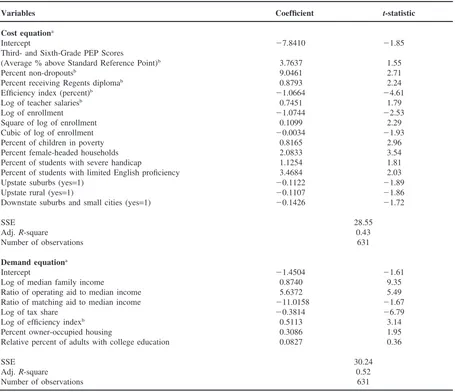
We estimate this model for 631 school districts in New York state in 1991; the detailed results are presented in Appendix A, Table 10.3In particular, we find that
edu-2 Another approach to controlling for omitted variables is to
use multiple years of data to difference out unobserved fixed district effects, that is, effects that do not vary over time. Downes and Pogue (1994) use a fixed-effects model to estimate educational costs in Arizona. However, given that many environmental cost factors change slowly over time, and indeed may not change at all in available data sets, fixed effects models may dramatically underestimate the influence of environmental factors on costs. In essence, the fixed-effect approach is con-servative in its estimate of cost differences across districts, because some cost variation is captured by the district fixed effects, which are not considered cost variables. To avoid this problem, we use data for a single year and incorporate several new variables, including dummy variables for type of school district and an efficiency index, to control for unobserved fac-tors.
3 For a more detailed explanation of our procedures, see
cational costs in New York state are influenced by the cost of the main input, namely teachers, and by five environmental cost factors: district enrollment, the per-centage of children in poverty, the perper-centage of house-holds headed by a single female, the percentage of stu-dents with limited English proficiency, and the percent of students with severe disabilities.4The estimated cost impact of teachers salaries recognizes that these salaries reflect not only labor market conditions, over which a school district has no control, but also a district’s gen-erosity in wage setting. Thus, we use an estimating pro-cedure that limits the impact of salaries to the variation associated with underlying labor market conditions.5The estimated impact of district enrollment is nonlinear. Fol-lowing many previous studies, we find that the relation-ship between cost per pupil and enrollment is U-shaped, with relatively high costs in both the smallest and the largest districts.6
On the basis of our regression results, we combine these input and environmental cost factors into a cost index, which indicates how much a district must spend to achieve the same performance (as measured by our index) as a district with average costs (see Duncombe & Yinger, 1997). Specifically, we hold outcomes, efficiency and regional dummy variables constant at the state average so that the index reflects variation in teacher salaries and environmental factors only. An index value of 100 indicates average cost, for example, whereas an index value of 200 indicates that a district must spend twice the average amount to obtain any given performance result. Cost indexes by type of district are
Instruments for the outcome variables come from the demand equation, and instruments for the efficiency index come from the efficiency equation. While recent research in education cost functions have employed more flexible functional forms (Callan & Santerre, 1990, and Gyimah-Brempong & Gyapong, 1992), we believe such models would add complexity without significant insight.
4 Other measures of disability, such as the percentage of
stu-dents with any form of disability, are available but we do not use them because they are influenced by school district policies regarding the identification of disabilities. See Lankford and Wyckoff (1996).
5 Specifically, three steps were taken. The teacher salary
index is based on teachers with only 1 to 5 years of experience which hopefully reflect more closely market wages. Second, differences in average experience, gender, tenure and education of teachers across districts was held constant. Finally, the salary index was treated as endogenous in the wage equation with the county manufacturing wage and the county population in 1990 used as instruments.
6 As indicated in Appendix A, Table 10, we actually estimate
a cubic relationship, which allows the U-shape to flatten out at the highest enrollment levels. This was done to accommodate New York City which has over 20 times the enrollment of the next largest district (Buffalo).
presented in Table 1. Upstate suburbs have the lowest average cost index at 91.6, and New York City has the highest cost index, namely 306.2. The three large upstate cities also have high costs, with an average index of 182. It should be pointed out that these indexes are not driven by New York City. A regression analysis that excludes New York City results in cost indexes, both for the City and for other districts, that are similar to the indexes in Table 1. In fact, such a regression actually results in a somewhat higher index for the City. The plain fact is that, as shown in Table 1, the City faces both high labor costs and the harshest educational environment in the state; its costs are relatively high no matter which sample is used for the regression analysis.7
2.3. The demand equation
A crucial step in understanding the impact of school aid systems on student performance, is estimating the response of voters and school districts to changes in fac-tors such as aid and community income. Voters can respond to an aid increase by asking for an improvement in educational performance or a reduction in school taxes. School officials may react to increased aid by being less diligent in their use of school funds, thus increasing inefficiency. While understanding the behavioral response to school aid is crucial to accurate predictions of its effects, the capacity for such simula-tions is often lacking among education analysts in state government.8
In constructing our behavioral model, we draw on the large literature on the demand for educational outcomes (see Inman, 1979; Rubinfeld, 1987; Ladd & Yinger, 1991). In particular, we employ the well-known median voter model, in which a district’s demand for educational
7 An alternative method of estimating educational cost
indi-ces is to focus on exogenous factors that affect the compen-sation which has to be paid to recruit equal quality teachers, or what are commonly called, compensating wage differentials. Chambers (1995) has estimated teacher cost indices for most school districts in the country using data from the NCES. While these indices reflect the higher teacher salaries required in large cities, they significantly underestimate cost variation because they do not reflect the additional teachers and other resources required to bring student performance up to a given standard when the educational environment is harsh. For example, the teacher salary index for New York City in 1990 using the Chambers estimates (where the state average for New York is set equal to 100) is 130. This compares to our index of 306 for New York City using a more comprehensive definition of education costs.
8 In New York state, for example, the state Department of
367
W.
Duncombe,
J.
Yinger
/
Economics
of
Education
Review
19
(2000)
363–386
Average characteristics of school districts by region and type, New York school districts, 1991
Downstate Upstate
Characteristic State average New York City Yonkers Small cities Suburbs Large cities Rural Small cities Suburbs
Per pupil expenditure
Unadjusted:
Total expenditures $8,399 $7,501 $10,001 $12,135 $11,874 $8,245 $7,472 $7,312 $7,402 Operating expenditures $6,058 $6,082 $6,781 $8,741 $9,016 $5,186 $5,145 $5,194 $5,333 Adjusted for cost:
Total expenditures $8,399 $2,450 $5,340 $9,202 $10,829 $4,529 $7,639 $6,686 $8,084
Operating expenditures $6,058 $1,986 $3,620 $6,629 $8,222 $2,849 $5,260 $4,749 $5,824
Fiscal capacity
Per pupil property value $367,160 $380,467 $460,621 $676,798 $798,868 $161,681 $243,810 $215,089 $261,175 Median family income $40,438 $34,360 $43,305 $54,635 $61,635 $26,527 $30,474 $32,518 $39,029 Local school property tax rateb 2 1.5 1.9 1.8 1.9 2.2 2.0 2.1 2.1
Cost and other factors
Cost index 100.0 306.2 187.3 131.9 109.7 182.0 97.8 109.4 91.6
Teacher salariesc $24,722 $27,227 $26,707 $28,714 $28,004 $25,753 $23,933 $23,370 $23,721 Enrollment 3,878 931,211 18,244 4,592 3,277 33,054 1,060 4,134 2,273 Percent of children in poverty 11.6 29.6 19.9 10.9 5.2 36.5 16.0 19.3 9.2 Percent female-headed households 8.8 18.1 15.7 12.3 9.3 19.1 8.2 11.7 8.2 Percent students with severe 4.5 6.3 10.0 7.1 5.3 7.8 4.1 5.6 4.0 handicaps
Percent students with limited 1.0 9.8 5.8 4.3 2.2 2.1 0.6 1.0 0.6 English
Population density 1,167.1 38,138.4 10,612.3 7,053.9 3,061.7 6,268.3 64.8 1,825.8 532.9
a The same sample of 631 districts was used in these calculations as in the other tables.
outcomes, as determined through voting, is a function of the median voter’s income, Y; the aid received by the district, A, the decisive voter’s tax price, TP; an efficiency index,e; and various preference variables, rep-resented byR.
S5f(Y,A,TP,e,R). (2)
Our demand model uses an index of the three outcomes discussed previously as the dependent variable.9 Prefer-ence variables include community characteristics, such as the percentage of adults who graduated from college and the percentage of households living in owner-occu-pied housing, that might affect voting outcomes.10
Following the literature (especially Ladd & Yinger, 1991), we define the tax price,TP, as the tax share multi-plied by the marginal expenditure for educational ser-vices. We measure the tax share with the ratio of median housing value to total property value per pupil. Marginal expenditure equals marginal cost divided by the efficiency index to reflect wasted spending. Assuming constant returns to scale with respect toS, an assumption used by virtually all education cost studies, average cost equals marginal cost, and the education cost index from the cost model can be used as a measure of marginal cost. In estimating the demand model, we split marginal expenditure into two pieces. The first piece is the tax share multiplied by the cost index and the second is the efficiency index. This procedure recognizes that voters may have different perceptions about, and hence differ-ent responses to, inefficiency and the tax share.
In addition, voter demand for educational performance depends on state aid; the higher the aid, the greater the
9 An alternative approach to estimating voter demand for
education is to estimate a system of demand equations for each individual performance indicator. This approach does not elim-inate the need to reduce the number of performance measures in the cost equation, nor does it provide much guidance on which outcomes measures to include. While the use of a simultaneous system of equations has been used for production functions (Boardman, Davis & Sanday, 1977), to the best of our knowl-edge, it has not been used to estimate education demand equa-tions. In theory it is possible to estimate a series of demand equations by the decisive voter for different educational per-formance measures (see Goldberger, 1987, for a review of demand system functional forms). However, such demand sys-tems would require measures of tax prices for each educational outcome. It may be possible to construct tax prices for broad classes of public services (Blackley & DeBoer, 1987), but this is not feasible for education.
10 Because of a high correlation between the percent of
col-lege graduates and median income, we used the residual from a regression of percent college on median income as the col-lege variable.
desired performance and spending.11 Although an increase in aid is similar to an increase in income, many studies have established that aid increases have a greater impact on district spending than do comparable increases in income. This is known as the flypaper effect; money “sticks where it hits”. We utilize the state aid variable in the demand equation to simulate how different types of aid systems affect voter demand for outcomes, spend-ing and tax rates.
The estimates of the demand model are consistent with findings of past studies of education demand (see Appen-dix A, Table 10).12The income elasticity for education is estimated to be somewhat below unity, 0.87, which is somewhat higher than that found in most past research (see Inman, 1979). This result may reflect the fact that, unlike previous studies, we control for costs and efficiency.13The coefficient for the operating aid is stat-istically significant and is consistent with the so called “fly-paper” effect. The price elasticity for education, m,
is estimated to be 20.38, which is in line with past
research on education (see Inman, 1979). In addition, the coefficient of the “efficiency” index is positive and stat-istically significant; as expected, higher efficiency lowers the effective price facing the median voter and increases demand for S. Of the preference variables we have included, only the percent owner-occupied housing has a significant positive relationship with educational out-comes.
2.4. The efficiency equation
The third equation examines the determinants of school district efficiency, as measured using a “best-practice” technique. With this technique, a district is said to be inefficient if it spends more on education than other districts with the same performance and the same edu-cational costs. The degree of inefficiency is measured by the extent of this excess spending. Although the “best-practice” technique we use, called data envelopment
11 The actual state aid variable included in the demand model
is the aid per pupil divided by median income and multiplied by the tax share. Aid is multiplied by the tax share to reflect the reduction in taxes on the median voter from an additional dollar of state aid. The term is divided by median income to reflect the actual budget constraint facing this voter (see Dun-combe & Yinger, 1998).
12 We estimate our demand model in log-linear form using
2SLS, with efficiency treated as endogenous. Instruments are derived from the efficiency equation. The aid variables and the preference factors are not expressed as logarithms.
13 When we estimate a median voter model without the cost
analysis or DEA, is well known, we are the first to use it in a comprehensive analysis of school district responses to educational policy reforms. As a result, this is the most exploratory part our analytical framework.
To keep our efficiency results in perspective, it is worth emphasizing that they depend both on our method for estimating efficiency and on our definition of per-formance. In other words, we explore the impact of vari-ous policy changes on best-practice efficiency in delivering educational performance as measured by our index. So far, scholars have not identified any other approach to estimating efficiency that can be employed in an analysis of school district behavior, but our approach is not without limitations (see Duncombe & Yinger, 1997), so further research on this topic clearly is warranted. Moreover, other scholars might prefer to apply our approach to efficiency to a different perform-ance index.
The literature on managerial efficiency and public bureaucracies suggests three broad factors that might by related to productive inefficiency: fiscal capacity, compe-tition, and factors affecting voter involvement in moni-toring government (see especially Leibenstein, 1966; Niskanen, 1971; Wyckoff, 1990; Duncombe, Miner & Ruggiero, 1997). First, the pressure put on school boards and school officials is influenced by the tightness of the budget constraint. Districts with higher income or pro-perty values tend to face less pressure to perform and hence have lower efficiency. Of particular importance for our simulation is the influence of state aid on efficiency. In particular, districts are more efficient if (a) they receive less aid per pupil than other districts in their enrollment/property value class or (b) if they are in an enrollment/property value class that receives a relatively low amount of aid per pupil.14Thus, districts make extra efforts to keep up with comparable districts that are receiving more aid and classes of district receiving the least aid are forced to find additional ways to cut their expenses without sacrificing performance. Using a tobit regression model, we find that all of these variables have the expected sign and most are statistically significant (see Appendix A, Table 11).15
14 The within class aid variable is mediated by the distance
a district’s enrollment is from the mean enrollment of a class.
15 The Tobit regression results are adjusted using the method
recommended by McDonald and Moffitt (1980) for values above the limit for use in the efficiency simulation. (Table 11 includes the adjusted beta coefficients.) Besides including efficiency variables, we have included other factors that could influence the DEA efficiency index. Since the DEA index, which compares per pupil expenditures and outcome measures, can be influenced by the environment in which education is provided, we control for the environmental factors in the cost model. Also, our measure of efficiency is based on the assump-tion that only the outcomes we look at are of value to voters.
Second, public choice scholars emphasize that compe-tition in the delivery of a public service is likely to put external pressure on managers to be more efficient. Com-petition can come in the form of comCom-petition from public and private schools, as well as voter referendums on dis-trict budgets. We have included measures of private school competition (percent of county students in private schools), public school competition (measure of public school concentration in a county), and the lack of a voter referendum (in city school districts).16None of the com-petition variables are statistically significant. This result contrasts with some other recent research indicating that competition improves performance (Hoxby, 1994a,b).
Finally, various characteristics of a school district may affect how much parents are willing and able to monitor the performance of their schools. We expect that in dis-tricts with more college educated parents and smaller geographic size parents will be more involved in public education and efficiency will be higher. While the vari-able for college educated adults is positive and signifi-cant, the coefficient on geographic area goes against expectations (although not significant at conventional levels). In addition, we hypothesize that efficiency is influenced by the share of any additional dollar of rev-enue that must be contributed by voters, which, as noted earlier, is called the tax share. The larger the tax share, the greater the bite that any tax increase takes out of voters’ pocketbooks, the more voter vigilance, and there-fore the higher the efficiency on the part of school administrators. Our empirical results in Table 11 strongly confirm this hypothesis.
2.5. Simulation methodology
These three equations allow us to simulate the impact of many different educational policies on educational performance, local tax rates, and school district
Since there may be variation in the outcome objectives across districts, we include a number of other outcome measures in the regression model. Finally, to control for possible omitted variables which may be correlated with the distinction between districts in upstate or downstate New York, we have included a dummy variable for downstate suburbs and small cities. This variable may be picking up omitted cost or outcome measures. These omitted outcomes and cost factors are held constant in constructing our estimates of the efficiency index in Table 9.
16 To measure concentration, we constructed a Herfendahl
efficiency. The cost equation is used to construct a cost index. As discussed more fully below, this cost index is a key element in the design of performance-based school aid systems. Changes in school aid influence educational performance both directly (through the aid effect) and indirectly (through their impact on efficiency). We use the efficiency equation to estimate this efficiency effect. Because aid variables and efficiency are factors in the voter demand model, we use this model to simulate how changes in aid influence the amount of educational per-formance voters demand. Using the cost index, the efficiency index, and the district property tax base, we estimate the spending level and property tax rates required to achieve the desired outcome level. Except where noted, our simulations also are budget neutral, in the sense that they simply redistribute the existing state aid budget.17
3. An analysis of performance standards
Educational performance standards are now under active discussion at both the national and the state level. New York State has long been a leader in this debate because of its Regents exams, which set implicit stan-dards for success in high school. Moreover, the recent implementation of district report cards in New York highlights each district’s performance and facilitates a discussion of the standards that each district should be expected to reach. The Regents have been exploring the possibility of issuing more explicit performance stan-dards, but have not yet determined whether to take this step, how to set these standards, or how to ensure that districts meet them.
The academic literature on standards is limited. One scholar, Bishop (1994), argues that clearly articulated standards can boost performance. In fact, on the basis of a statistical analysis of SAT scores in the United States, Bishop argues that the relatively high performance on SATs of students in New York state can be attributed in part to the existence of Regents exams.18
A full analysis of performance must consider many issues. How can a system of standards avoid encouraging schools to “teach to the test”? Will a standard imposed on one performance indicator, such as Regents diplomas, lead to poorer performance on competing indicators,
17 Our simulations are based on the 1991 state aid budget.
We include the following programs, which had a total cost of $5.7 billion: Operating Aid, Attendance Improvement–Dropout Prevention Aid, High Tax Aid, Limited English Proficiency Aid, Compensatory Education Needs Aid, Compensatory Edu-cation Needs Aid–Small Cities, Small City Aid, EduEdu-cationally Related Support Services Aid, and Supplemental Support Aid.
18 See also Costrell (1994), and Kang (1985).
such as the graduation rate, or to accompanying perform-ance increases on complementary indicators, such as scores on elementary school tests. (In New York, the principal tests taken in elementary schools are the PEP tests for reading and math in 3rd and 6th grades.) This type of full analysis is beyond the scope of this paper. Instead, we will use our analytical framework to explore the magnitude of the task facing school districts and state policy makers if they want to bring low-performing dis-tricts up to a higher standard.
3.1. How can a district meet a performance standard?
Acting on its own, the only ways for a low-performing school district to reach a performance standard are (1) to raise its property tax rate and use the funds to purchase better performance, (2) to improve the efficiency with which it uses its resources, or (3) some combination of the two. Our analytical framework does not allow us to determine how districts can find the political resources needed to raise their tax rates, nor does it show how they can improve their management practices so as to be more efficient. However, this framework does reveal the extent of the tax-rate or efficiency changes that would be neces-sary to meet a general performance standard.
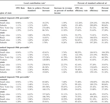
We focus on operating spending, not total spending, and define the “local contribution rate” as the tax rate levied by a district in support of its operating budget. We then examine the increase in this tax rate required to bring each district up to three given standards, namely the 25th, 50th, and 75th percentiles of the current per-formance distribution, as measured by our perper-formance index. Recall that this index is based on elementary test scores, Regents diplomas, and graduation rates. Obvi-ously, districts with higher costs (or higher inefficiency) will have to spend more to obtain any given increase in performance, districts that are far from the standard will have to spend more to reach it than other districts, and districts with relatively small property tax bases will have to raise their tax rates more than districts with rela-tively large bases.
Table 2
Comparison of local contribution rate and efficiency rate required to achieve an outcome standard with the 1991 aid distribution. Averages by region for New York school districts, 1991a
Local contribution rateb Percent of standard achieved atc
1991 Rate Rate to achieve Percent Increase in revenue 1991 est. Full Percent standard increase as percent of median efficiency rate efficiency incease
Region of state income
Standard imposed–25th percentiled Downstate
Small cities 0.94% 1.12% 18.23% 1.39% 112.26% 229.24% 104.20%
Suburbs 1.11% 1.21% 8.89% 0.60% 151.48% 289.09% 90.84%
New York City 1.01% 3.79% 274.48% 30.73% 33.41% 53.72% 60.79%
Yonkers 1.29% 2.41% 86.74% 11.92% 37.63% 51.63% 37.20%
Upstate
Large cities 1.51% 3.88% 156.55% 14.91% 52.27% 71.01% 35.87%
Rural 1.08% 1.23% 14.01% 0.89% 115.42% 166.92% 44.61%
Small cities 1.19% 1.69% 42.66% 2.87% 94.82% 139.29% 46.91%
Suburbs 1.20% 1.24% 3.70% 0.28% 130.49% 197.28% 51.18%
Standard imposed–50th percentiled Downstate
Small cities 0.94% 1.37% 45.61% 3.74% 90.55% 184.91% 104.20%
Suburbs 1.11% 1.30% 17.61% 1.38% 122.19% 233.19% 90.84%
New York City 1.01% 4.78% 373.28% 41.79% 26.95% 43.33% 60.79%
Yonkers 1.29% 2.84% 120.08% 16.50% 30.35% 41.65% 37.20%
Upstate
Large cities 1.51% 5.13% 238.81% 22.27% 42.16% 57.28% 35.87%
Rural 1.08% 1.58% 46.36% 2.71% 93.11% 134.64% 44.61%
Small cities 1.19% 2.26% 90.80% 6.12% 76.48% 112.36% 46.91%
Suburbs 1.20% 1.42% 19.04% 1.26% 105.26% 159.14% 51.18%
Standard imposed–75th percentiled Downstate
Small cities 0.94% 1.75% 85.68% 7.40% 73.48% 150.05% 104.20%
Suburbs 1.11% 1.48% 33.41% 2.87% 99.16% 189.23% 90.84%
New York City 1.01% 5.98% 491.98% 55.07% 21.87% 35.16% 60.79%
Yonkers 1.29% 3.36% 160.13% 22.00% 24.63% 33.80% 37.20%
Upstate
Large cities 1.51% 6.63% 337.64% 31.11% 34.21% 46.49% 35.87%
Rural 1.08% 2.23% 106.79% 6.08% 75.55% 109.26% 44.61%
Small cities 1.19% 3.06% 158.01% 10.59% 62.06% 91.18% 46.91%
Suburbs 1.20% 1.86% 55.91% 3.57% 85.42% 129.14% 51.18%
a The number of districts used in these calculations is 631. Missing data existed for the other districts which were predominantly
small school districts.
b The local contribution rate is calculated by subtracting per pupil lump-sum aid from operating expenditures and dividing by per
pupil property values.
c The fifth column is calculated by taking the ratio of actual performance under the present aid system and the performance level
associated with each standard. The sixth column is the ratio of estimated performance with no relative inefficiency compared to the standard.
d Percentiles refer to the 1991 distribution for outcomes based on a composite index of three outcomes: percent of students receiving
upstate large city districts would have to raise rates 157 percent. The fourth column of Table 2 reveals that the required tax increases in large cities also would be rela-tively high if expressed as a percentage of a district’s median income. For example, New York City would need to raise taxes per pupil equivalent to 31 percent of the median family income. This compares to tax burdens of less than 2 percent of income in most other districts.19 The next two panels examine higher standards. In the last panel, which refers to a standard set at the 75th per-centile of the 1991 performance distribution, all districts except suburbs and downstate small cities would have to at least double their tax rates to meet the standard, and New York City would have to increase its rate by 492 percent. As before the required tax increases also are a relatively high percentage of income in large cities; indeed, expressed this way the increase is almost 15 times as high in New York City as in its suburbs. The required tax rate increase in New York City would have to be impossibly high, 55 percent of median family income.
The second possibility mentioned above is for districts to become more efficient. We address this issue by rais-ing the efficiency of all low-performrais-ing districts up to the highest level observed in current practice. It is theor-etically possible for efficiency improvements beyond this point to be obtained, but since they would be outside the experience of any district in the state, we do not examine them. The results are presented in the last three columns of Table 2. Small, downstate cities, for example, now average 112.3 percent of the first performance target. If these districts were all “perfectly” efficient, they would exceed the 25th percentile performance target by over two times, on average. All types of districts except large cities exceed the standard with present efficiency, and would be more than 40 percent above the standard with full efficiency. In contrast, New York City and Yonkers now reach about 30 percent of this minimal performance standard, but would just reach half of this standard if they were as efficient as current practice allows. Similar efficiency improvements would bring the large upstate cities only up to 70 percent of the standard. The next two panels of this table reveal that efficiency changes alone continue to bring most districts up to the higher performance standards except for the large cities. For example, best-practice efficiency would not bring New York City and Yonkers even up to 36 percent of the highest standard.
19 Some might prefer this alternative method for calculating
the burden because, unlike the percentage increase in the pro-perty tax rate, it is not affected by the types of taxes a district uses—or shares with other governmental activities. It is not affected, for example, by the income tax in New York City.
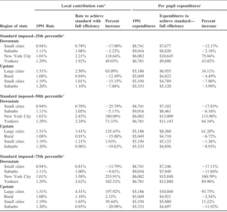
Table 3 presents estimates of the required tax rates and expenditure levels to achieve a given standard if a district is assumed to be fully efficient. With full efficiency the tax increase required to reach a standard in the large cities is sixty to seventy percent of what it is at present efficiency levels. For New York City to reach the 25th percentile, for example, would require an increase in the local contribution rate of 119 percent compared to 274 percent under present efficiency levels (refer to column 3 in Table 2 and Table 3). The last three columns of this table present the spending levels required to reach the standard under full efficiency. For New York City to achieve the 25th percentile of the 1991 perform-ance distribution would require a 75 percent increase in expenditures, and to reach the 75th percentile would require expenditure increase of more than 2.5 times. To keep these spending increases in perspective, note that they result in performance increases of 3 and 4.5 times, respectively, over 1991 levels.
3.2. Can a revised state aid program help districts meet a performance standard?
3.2.1. Aid system design
A performance standard might induce low-performing districts to boost their performance by raising their taxes or improving their efficiency, but given the magnitude of the required changes, it seems unlikely that such efforts would be sufficient to reach the standards. An alternative, to which we now turn, is to combine a per-formance standard with aid changes designed to ensure that every district has the resources needed to meet it.
The type of aid program we consider is called a foun-dation plan and is used by 80 percent of the states, including New York.20 However, our foundation plan, unlike the actual plan in any state, systematically accounts for cost differences across districts. Existing plans, including New York’s, are designed to bring all districts up to a minimum spending level per pupil. Let
Vistand for the property tax base in district i, then an expenditure-based foundation grant per pupil is defined by
Ai5E∗2t∗Vi5E∗(12vi), (3) where E* is the expenditure standard,t* is the state set minimum tax rate,V*=E*/t* is the property value above which a district receives no aid andviis a property value
20 Historically, New York has used a modified foundation
Table 3
Comparison of local contribution rate and per pupil operating expenditures required to achieve an outcome standard with the 1991 aid distribution. Averages by region for New York school districts, 1991a
Local contribution rateb Per pupil expendituresc
Rate to achieve Expenditures to
standard with Percent 1991 achieve standard— Percent Region of state 1991 Rate full efficiency increase expenditures full efficiency increase
Standard imposed–25th percentiled Downstate
Small cities 0.94% 0.78% 217.00% $8,741 $7,677 212.17%
Suburbs 1.11% 1.08% 22.22% $9,016 $8,820 22.18%
New York City 1.01% 2.21% 118.64% $6,082 $10,645 75.04%
Yonkers 1.29% 1.92% 49.03% $6,781 $9,698 43.02%
Upstate
Large cities 1.51% 2.50% 65.09% $5,186 $6,955 34.11%
Rural 1.08% 0.94% 212.49% $5,049 $4,823 24.49%
Small cities 1.19% 1.01% 215.15% $5,194 $4,789 27.80%
Suburbs 1.20% 1.10% 27.88% $5,333 $5,120 23.99%
Standard imposed–50th percentiled Downstate
Small cities 0.94% 0.70% 225.79% $8,741 $7,182 217.83%
Suburbs 1.11% 1.05% 25.17% $9,016 $8,461 26.16%
New York City 1.01% 2.83% 180.09% $6,082 $13,009 113.90%
Yonkers 1.29% 2.24% 73.33% $6,781 $11,143 64.34%
Upstate
Large cities 1.51% 3.41% 125.43% $5,186 $8,360 61.20%
Rural 1.08% 0.91% 215.88% $5,049 $4,710 26.72%
Small cities 1.19% 1.21% 1.63% $5,194 $5,123 21.36%
Suburbs 1.20% 0.96% 219.62% $5,333 $4,856 28.93%
Standard imposed–75th percentiled Downstate
Small cities 0.94% 0.81% 213.79% $8,741 $7,246 217.11%
Suburbs 1.11% 1.00% 29.81% $9,016 $7,949 211.84%
New York City 1.01% 3.58% 253.91% $6,082 $15,848 160.59%
Yonkers 1.29% 2.62% 102.52% $6,781 $12,880 89.96%
Upstate
Large cities 1.51% 4.51% 197.92% $5,186 $10,048 93.75%
Rural 1.08% 1.10% 2.32% $5,049 $4,921 22.54%
Small cities 1.19% 1.65% 39.44% $5,194 $5,880 13.22%
Suburbs 1.20% 0.95% 220.98% $5,333 $4,697 211.92%
a The number of districts used in these calculations is 631. Missing data existed for the other districts which were predominantly
small school districts.
b The local contribution rate is calculated by subtracting per pupil lump-sum aid from operating expenditures and dividing by per
pupil property values.
c Expenditures are based on approved operating expenditures.
d Percentiles refer to the 1991 distribution for outcomes based on a composite index of three outcomes: percent of students receiving
a Regents Diploma, percent of students not dropping out, and average percent of students above the state set standard reference point for 3rd and 6th grade PEP tests.
index. A foundation aid program is designed to provide every district with enough resources to provide the foun-dation level of spending per pupil at a tax ratet* speci-fied by policy makers. Districts that are wealthy enough to raise the required revenue by themselves simply by
is usually modified in practice, through minimum aid amounts or hold-harmless clauses, so that all districts receive some aid, thereby reducing the equalizing power of the formula. Moreover, a foundation grant usually is accompanied by a requirement that each district levy a tax rate of at leastt*; otherwise, some districts might not provide the minimum acceptable spending level, E*. New York and Illinois are notable exceptions; see Miner (1991) and Downes and McGuire (1994).
Because they do not systematically account for cost differences across districts, these plans do not bring all districts up to a minimum performance level (Duncombe & Yinger, 1997). Moreover, many existing foundation plans, again including New York’s, have hold-harmless provisions or minimum aid amounts that limit their ability to bring all districts up to an adequate spending level per pupil, let alone adequate performance. Our aid programs do not contain any such provisions. We make the switch from spending to performance by bringing in the cost index derived from our estimated cost equation into the aid formula. This index allows us to determine how much a district with a certain cost level would have to spend to achieve a performance target. To bring all districts up to a performance standard, denoted byS*, at an acceptable tax burden on their residents, the outcome-basedfoundation formula should be
Ai5S∗Ci2t∗Vi5E∗(ci2vi), (4) whereCiis the amount the district must spend to obtain one unit ofS (per unit cost), andciand viare cost and property value indices (Ladd & Yinger, 1994). The amount of aid this district receives equals the spending level required to reachS* minus the amount of revenue it can raise at the specified tax ratet*. As with Eq. (3), raisingS* to an extremely high level would, at great cost, result in an equal educational output in every district, and allowing negative grants would boost the equalizing impact of the grant.
The 1996 New York State aid programs include sev-eral provisions that could be interpreted as ad hoc cost adjustments. The first is that operating aid, which pro-vides 53 percent of the total aid paid to school districts, is based on the number of “weighted” pupils in a district. Pupils with extra weights include pupils in secondary school and pupils with “special education needs”, defined as students who score below the minimum com-petency level on the third and sixth grade reading or math PEP tests.21The first of these weighting factors is supported by some studies of school spending in other states (see, for example, Ratcliffe et al., 1990), which
21 The other two weighting factors bring in students not
coun-ted in average daily attendance, namely students in half-day kindergarten (with a weight of 0.5) and students in summer school (with a weight of 0.12).
find a higher cost for high school than for elementary school students. However, it is not supported by our analysis of data for New York state, which finds no cost differences by grade. The second factor is undoubtedly correlated with cost variables, but we believe it is inap-propriate to include a performance measure based on PEP scores in an aid formula. This approach rewards districts for poor performance and gives them an incen-tive to perform poorly in the future. Aid formulas should be based on factors outside a district’s control, such as concentrated poverty, that make it difficult for the district to reach a high performance standard, not on perform-ance indicators that are influenced by the district’s actions. New York also has a relatively new program, called Extraordinary Needs Aid, which gives more aid to districts with lower incomes and higher poverty con-centrations. The program provides less than 5 percent of the total aid budget, and the formula is ad hoc, that is, it is not based on any estimate of the relationship between educational costs and poverty. Overall, therefore, these programs do a poor job accounting for cost differences across districts.22
Even with an aid program that accurately accounts for cost factors, a district can fall short of the foundation level of spending or performance either because it is inefficient or because it sets a tax rate that is below the specified rate. Because virtually all districts fall short of the best-practice efficiency level, we design our foun-dation formula so that every district will have enough revenue to achieve the foundation performance level if it at least reaches the 75th percentile of the current efficiency distribution across districts, which we call the baseline efficiency level. If it falls short of this level, it will not achieve the foundation level of performance unless its tax rate is above the specified rate.
3.2.2. Aid simulations
Using data on New York school districts in 1991, we simulate the effect of different aid systems on student outcomes, district expenditures, tax rates and efficiency. We examine aid programs without negative aid and with three different performance standards, namely the 25th, 50th, and 75th percentiles of the 1991 performance dis-tribution in New York, as measured by our outcome
22 New York State also provides aid for transportation and
index. As we illustrate below, the impact of these aid programs depends primarily on four key issues:
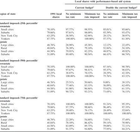
First, additional aid makes it possible for a district to maintain its current service level while cutting back on local property taxes. Foundation plans are supposed to be accompanied by a required minimum local tax rate to prevent such a cut back. Without a minimum-tax-rate provision, as is the case in New York, the stimulative impact of state aid is minimal. We examine aid programs with and without a minimum-tax-rate provision. Our ver-sion of the minimum-tax-rate proviver-sion has two parts. (a) All districts that receive foundation aid must set their tax rate at or above the rate specified in the foundation formula. (b) All districts that are too wealthy to receive foundation aid must set their tax rate at or above the rate required for them to reach the foundation level of performance at the baseline level of efficiency. This minimum rate will be below the rate imposed on districts that actually receive foundation aid.
Second, performance is influenced by the generosity of the state aid program. As explained earlier, aid raises voters’ desired performance level and hence raises school district performance. However, additional aid does not simply go into higher performance, it also leads to local tax reductions, so the impact of aid on perform-ance may not be large. We examine aid programs using the 1990–91 New York State aid budget and twice this amount. Note that these first two issues interact because the generosity of the state aid program determines the property tax rate needed to reach any performance target; the more generous the aid, the lower the required rate.
Third, as explained earlier, aid programs influence school district efficiency. In general, the more aid a dis-trict receives, the less efficient it will be. Thus, a policy to improve the performance of low-performing school districts with more state aid is analogous to a leaky bucket; some of the aid these districts receives is lost in the form of higher managerial inefficiency. This prin-ciple applies not only to a redistribution of aid toward needier districts, which makes those districts less efficient, but also to an increase in the state aid budget with a given formula, which makes all districts less efficient. We are not, of course, the first scholars to point to the leaks in the aid bucket, and in fact some scholars think that it is much leakier than we do (see Hanu-shek, 1996).
Fourth, the impact of any aid program in New York state is heavily influenced by the situation in New York City. Because New York City is such a needy district, with both the highest costs in the state and relatively low property value per pupil, any redistribution toward the neediest districts will increase New York City’s aid per pupil. Moreover, because New York City has such a high enrollment, any increase in its aid per pupil will consume a large share of the state aid budget. At the current time, New York State deals with this issue by giving New
York City significantly less aid per pupil than it gives the average district ($2,747 compared to $3,623 in 1995– 96; see The University of the State of New York, 1997). In contrast, our aid systems are driven by the principle that all districts should be brought up to a minimum per-formance standard, so New York City’s aid per pupil is above average and less is left over for other districts. This effect may arise for large cities in other states, but undoubtedly not to the same degree.
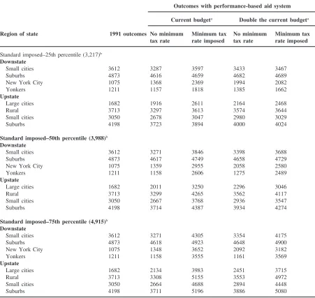
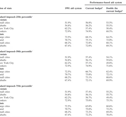
Table 4 presents our predicted performance for each type of school district under various aid plans. The col-umns refer to the two different state budget levels and to plans with and without a minimum-tax-rate require-ment. The three panels refer to the three different stan-dards. Outcomes in 1991, based on our index, are given in the first column.
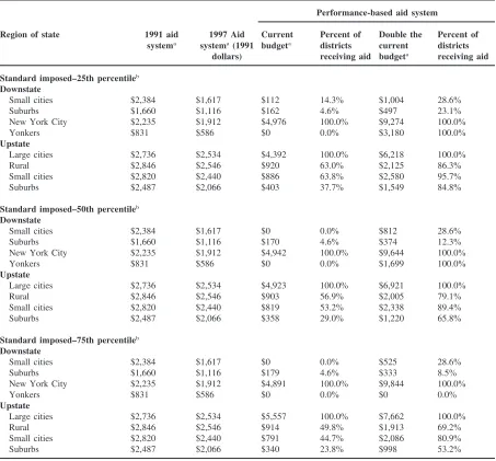
A comparison of the first and second columns indi-cates that changing from the current aid formula to a performance-based foundation plan with no minimum tax rate would actually lower outcomes in all types of districts except New York City and the upstate large cit-ies. This result reflects the facts that a performance-based aid program, unlike the current one, recognizes the high costs and low capacity of New York City and that raising the aid per pupil to the City uses up a large share of the state aid budget. In fact, as shown in Table 5, aid per pupil declines in all classes of district except for these large cities, and indeed declines to zero in many districts. For example, 14 percent of the downstate small cities and only 5 percent of the downstate suburban districts would receive operating aid.
Imposing a minimum tax rate, in the third column of Table 4, enlists each school district in the effort to reach the performance standard. Because the state aid budget is relatively ungenerous and so much money flows to New York City, the required local contribution is very large. Table 6 shows that a minimum-tax-rate require-ment results in a higher local tax rate, on average, in every class of district. Not surprisingly, low-performing districts, such as the big cities, face particularly large rate increases. In fact, New York City and most of the upstate big cities are pushed all the way to the minimum tax rate in the foundation formula, which, for the highest standard, is over four times the current New York City tax rate.
Table 4
Comparison of predicted outcomes with different budget levels and aid systems. 1991 aid system compared to performance-based foundation aid formula (with minimum aid level set at zero). Averages by region for New York school districts, 1991
Outcomes with performance-based aid system
Current budgeta Double the current budgeta
Region of state 1991 outcomes No minimum Minimum tax No minimum Minimum tax tax rate rate imposed tax rate rate imposed
Standard imposed–25th percentile (3,217)b Downstate
Small cities 3612 3287 3597 3433 3467
Suburbs 4873 4616 4659 4682 4689
New York City 1075 1368 2369 1994 2082
Yonkers 1211 1157 1818 1385 1662
Upstate
Large cities 1682 1916 2611 2164 2468
Rural 3713 3297 3613 3574 3644
Small cities 3050 2678 3047 2980 3029
Suburbs 4198 3723 3894 4000 4024
Standard imposed–50th percentile (3,988)b Downstate
Small cities 3612 3271 3846 3398 3688
Suburbs 4873 4617 4749 4658 4729
New York City 1075 1359 2955 2058 2580
Yonkers 1211 1158 2606 1275 2489
Upstate
Large cities 1682 2011 3250 2296 3046
Rural 3713 3299 4265 3562 4117
Small cities 3050 2667 3768 2936 3547
Suburbs 4198 3714 4387 3934 4274
Standard imposed–75th percentile (4,915)b Downstate
Small cities 3612 3271 4305 3354 4175
Suburbs 4873 4618 4923 4648 4900
New York City 1075 1348 3652 2092 3182
Yonkers 1211 1158 3555 1161 3569
Upstate
Large cities 1682 2134 3983 2451 3715
Rural 3713 3308 5155 3553 4972
Small cities 3050 2664 4688 2894 4448
Suburbs 4198 3711 5196 3886 5080
a The aid budget includes eight forms of aid besides operating aid (see note 17 in the text). The state aid budget for the 631
districts in our sample was $5.7 billion in 1991.
b Percentiles refer to the 1991 distribution for outcomes based on a composite index of three outcomes: percent of students receiving
a Regents Diploma, percent of students not dropping out, and average percent of students above the state set standard reference point for 3rd and 6th grade PEP tests.
the 50 percentile standard, New York City almost reaches the 25th percentile standard, which is three times the City’s actual performance in 1991.
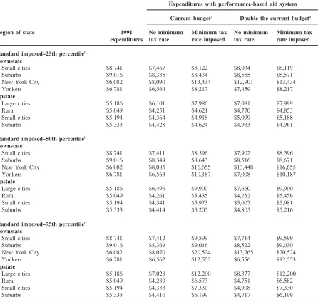
A performance-based foundation aid plan with the 1991 state aid budget and no required minimum tax rate would also lower spending for all classes of districts, except for New York City and the large upstate cities
(columns 1 and 2 in Table 7).23Doubling the state aid budget would lead to expenditure increases in large cit-ies, but expenditures would remain below 1991 levels in most other districts because the performance-based aid
per-Table 5
Comparison of aid per pupil under different budget levels and aid systems. 1991 aid system compared to performance-based foundation aid formula (with minimum aid level set at zero). Averages by region for New York school districts (1991 dollars)
Performance-based aid system
Region of state 1991 aid 1997 Aid Current Percent of Double the Percent of systema systema(1991 budgeta districts current districts
dollars) receiving aid budgeta receiving aid
Standard imposed–25th percentileb Downstate
Small cities $2,384 $1,617 $112 14.3% $1,004 28.6%
Suburbs $1,660 $1,116 $162 4.6% $497 23.1%
New York City $2,235 $1,912 $4,976 100.0% $9,274 100.0%
Yonkers $831 $586 $0 0.0% $3,180 100.0%
Upstate
Large cities $2,736 $2,534 $4,392 100.0% $6,218 100.0%
Rural $2,846 $2,546 $920 63.0% $2,125 86.3%
Small cities $2,820 $2,440 $886 63.8% $2,580 95.7%
Suburbs $2,487 $2,066 $403 37.7% $1,549 84.8%
Standard imposed–50th percentileb Downstate
Small cities $2,384 $1,617 $0 0.0% $812 28.6%
Suburbs $1,660 $1,116 $170 4.6% $374 12.3%
New York City $2,235 $1,912 $4,942 100.0% $9,644 100.0%
Yonkers $831 $586 $0 0.0% $1,699 100.0%
Upstate
Large cities $2,736 $2,534 $4,923 100.0% $6,921 100.0%
Rural $2,846 $2,546 $903 56.9% $2,005 79.1%
Small cities $2,820 $2,440 $819 53.2% $2,338 89.4%
Suburbs $2,487 $2,066 $358 29.0% $1,220 65.8%
Standard imposed–75th percentileb Downstate
Small cities $2,384 $1,617 $0 0.0% $525 28.6%
Suburbs $1,660 $1,116 $179 4.6% $333 8.5%
New York City $2,235 $1,912 $4,891 100.0% $9,844 100.0%
Yonkers $831 $586 $0 0.0% $0 0.0%
Upstate
Large cities $2,736 $2,534 $5,557 100.0% $7,662 100.0%
Rural $2,846 $2,546 $914 49.8% $1,913 69.2%
Small cities $2,820 $2,440 $791 44.7% $2,086 80.9%
Suburbs $2,487 $2,066 $340 23.8% $998 53.2%
a The aid budget includes eight forms of aid besides operating aid (see note 17 in the text). The state aid budget for the 631
districts in our sample was $5.7 billion in 1991 dollars.
b Percentiles refer to the 1991 distribution for outcomes based on a composite index of three outcomes: percent of students receiving
a Regents Diploma, percent of students not dropping out, and average percent of students above the state set standard reference point for 3rd and 6th grade PEP tests.
formance distribution, outcomes and expenditures for New York City increase approximately 2.2 times. In fact, the out-come elasticity is one; a one percent increase in expenditures leads to a one percent increase in outcomes.
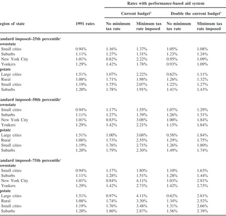
Table 6
Comparison of local contribution rates to operating expenditures under different budget levels and aid systems.a1991 aid system
compared to performance-based foundation aid formula (with minimum aid level set at zero). Averages by region for New York school districts, 1991
Rates with performance-based aid system
Current budgetb Double the current budgetb
Region of state 1991 rates No minimum Minimum tax No minimum Minimum tax
tax rate rate imposed tax rate rate imposed
Standard imposed–25th percentilec Downstate
Small cities 0.94% 1.16% 1.37% 1.05% 1.08%
Suburbs 1.11% 1.27% 1.31% 1.23% 1.24%
New York City 1.01% 0.82% 2.22% 0.95% 1.09%
Yonkers 1.29% 1.42% 1.78% 0.93% 1.09%
Upstate
Large cities 1.51% 1.07% 2.22% 0.62% 1.11%
Rural 1.08% 1.71% 1.98% 1.26% 1.32%
Small cities 1.19% 1.75% 2.07% 1.22% 1.27%
Suburbs 1.20% 1.78% 1.91% 1.41% 1.43%
Standard imposed–50th percentilec Downstate
Small cities 0.94% 1.17% 1.55% 1.07% 1.29%
Suburbs 1.11% 1.27% 1.39% 1.26% 1.31%
New York City 1.01% 0.83% 3.08% 1.00% 1.84%
Yonkers 1.29% 1.42% 2.21% 1.15% 1.84%
Upstate
Large cities 1.51% 1.00% 3.08% 0.58% 1.84%
Rural 1.08% 1.73% 2.55% 1.29% 1.75%
Small cities 1.19% 1.76% 2.71% 1.26% 1.80%
Suburbs 1.20% 1.79% 2.30% 1.49% 1.74%
Standard imposed–75th percentilec Downstate
Small cities 0.94% 1.17% 1.80% 1.10% 1.63%
Suburbs 1.11% 1.28% 1.51% 1.28% 1.44%
New York City 1.01% 0.84% 4.11% 1.03% 2.81%
Yonkers 1.29% 1.42% 2.73% 1.42% 2.73%
Upstate
Large cities 1.51% 0.97% 4.11% 0.62% 2.81%
Rural 1.08% 1.74% 3.30% 1.34% 2.52%
Small cities 1.19% 1.76% 3.48% 1.31% 2.66%
Suburbs 1.20% 1.80% 2.87% 1.56% 2.39%
a The local contribution rate is calculated by subtracting per pupil lump-sum aid from operating expenditures and dividing by per
pupil property values.
b The aid budget includes eight forms of aid besides operating aid (see note 17 in the text). The state aid budget for the 631
districts in our sample was $5.7 billion in 1991.
c Percentiles refer to the 1991 distribution for outcomes based on a composite index of three outcomes: percent of students receiving
a Regents Diploma, percent of students not dropping out, and average percent of students above the state set standard reference point for 3rd and 6th grade PEP tests.
is raised to the 75th percentile of 1991 outcomes, most districts would be forced to raise their tax rates compared to 1991, and, thus, their spending levels would generally equal or exceed 1991 levels, despite significant reductions in their state aid.
Table 7
Comparison of predicted operating expenditures per pupil with different budget levels and aid systems. 1991 aid system compared to performance-based foundation aid formula (with minimum aid level set at zero). Averages by region for New York school dis-tricts, 1991
Expenditures with performance-based aid system
Current budgeta Double the current budgeta
Region of state 1991 No minimum Minimum tax No minimum Minimum tax
expenditures tax rate rate imposed tax rate rate imposed
Standard imposed–25th percentileb Downstate
Small cities $8,741 $7,467 $8,122 $8,034 $8,119
Suburbs $9,016 $8,335 $8,434 $8,555 $8,571
New York City $6,082 $8,090 $13,434 $12,901 $13,434
Yonkers $6,781 $6,564 $8,217 $7,459 $8,217
Upstate
Large cities $5,186 $6,101 $7,986 $7,081 $7,999
Rural $5,049 $4,251 $4,621 $4,770 $4,853
Small cities $5,194 $4,364 $4,918 $5,099 $5,188
Suburbs $5,333 $4,428 $4,624 $4,933 $4,961
Standard imposed–50th percentileb Downstate
Small cities $8,741 $7,411 $8,596 $7,902 $8,596
Suburbs $9,016 $8,349 $8,643 $8,516 $8,671
New York City $6,082 $8,085 $16,655 $13,448 $16,655
Yonkers $6,781 $6,563 $10,187 $7,008 $10,187
Upstate
Large cities $5,186 $6,496 $9,900 $7,660 $9,900
Rural $5,049 $4,261 $5,435 $4,752 $5,456
Small cities $5,194 $4,341 $5,973 $5,007 $5,981
Suburbs $5,333 $4,414 $5,205 $4,805 $5,216
Standard imposed–75th percentileb Downstate
Small cities $8,741 $7,412 $9,599 $7,714 $9,599
Suburbs $9,016 $8,369 $9,016 $8,522 $9,030
New York City $6,082 $8,070 $20,524 $13,765 $20,524
Yonkers $6,781 $6,562 $12,553 $6,556 $12,553
Upstate
Large cities $5,186 $7,028 $12,200 $8,377 $12,200
Rural $5,049 $4,289 $6,573 $4,751 $6,582
Small cities $5,194 $4,333 $7,330 $4,908 $7,330
Suburbs $5,333 $4,410 $6,199 $4,717 $6,199
a The aid budget includes eight forms of aid besides operating aid (see note 17 in the text). The state aid budget for the 631
districts in our sample was $5.7 billion in 1991.
b Percentiles refer to the distribution for outcomes based on a composite index of three outcomes: percent of students receiving
a Regents Diploma, percent of students not dropping out, and average percent of students above the state set standard reference point for 3rd and 6th grade PEP tests.
formula). Similarly, it would cost taxpayers in the 399 districts below the median of the 1991 performance dis-tribution about $10 billion in additional local taxes to bring all districts near the middle performance standard, and about $15 billion in additional revenues to bring up the 541 districts falling below the highest performance