ANALYSIS
Is energy cost an accurate indicator of natural resource
quality?
David I. Stern *
Centre for Resource and En6ironmental Studies,The Australian National Uni6ersity,Canberra ACT0200,Australia Received 16 July 1997; received in revised form 8 February 1999; accepted 21 May 1999
Abstract
The use of energy cost as an indicator of natural resource quality is examined. Energy cost is the direct and indirect energy used to produce a unit of a resource commodity. Different approaches to the role of energy in the economy are discussed and it is demonstrated theoretically that energy cost can give false indications of changes in resource quality. This is because energy cost is only an accurate indicator of resource quality if either energy is the single primary factor of production and the economy can be represented by an input – output model, or if there is substitutability between the factors of production, then marginal products must be proportional to the factors’ embodied energy. These conditions are tested empirically using data from the US agricultural sector. The results show that there is substitutability and marginal products are not proportional to embodied energy. However, the strong neoclassical assumption of price-taking profit-maximization can be rejected at a 5% level of significance, though not at the 3.5% level. The generality of the empirical results may be restricted due to data limitations but the theoretical framework can be applied to other data sets, other resources, and even other indicators. © 1999 Elsevier Science B.V. All rights reserved.
Keywords:Resource quality; Energy cost; Energy analysis; Scarcity; Indicators
www.elsevier.com/locate/ecolecon
1. Introduction
This paper critically examines the basis for, and appropriateness of, energy cost as an indicator of natural resource quality. Energy cost is the amount of direct and indirect energy required to extract and process a unit of a resource to a given
standard. Energy cost has been used by some energy analysts as an indicator of natural resource quality (e.g. Cook, 1976; Chapman and Roberts, 1983; Hall et al., 1986; Cleveland, 1991). Resource quality is the productivity of the resource stock when all controlled inputs such as capital, labor, and energy are held constant. Changes in produc-tivity are then either the result of improved tech-nology or changes in the natural environment. Resource quality is an indicator of natural
re-* Tel.: +61-2-6249-0664; fax:+61-2-6249-0757. E-mail address:[email protected] (D.I. Stern)
source scarcity in that it indicates the use value capable of being generated by the resource stock (Cleveland and Stern, 1999).
Theoretical and empirical arguments are pre-sented, indicating that energy cost can be a mis-leading indicator, showing increasing scarcity while resource quality is actually increasing, and vice versa. The theory shows that if energy is the primary factor of production and the economy can be represented by an input – output model, then energy cost is an accurate indicator of re-source quality. When there is substitutability be-tween the factors of production, energy cost is only accurate when marginal products are propor-tional to factors’ embodied energy. Using data from the US agricultural sector, the evidence is in favor of substitutability with marginal products not proportional to embodied energy. Evidence for full neoclassical price-taking, profit-maximiz-ing behavior is less strong. The generality of the empirical results may be restricted due to data limitations. The available embodied energy time series data are not as systematically calcu-lated or as comprehensive as some cross-section estimates of embodied energy (e.g. Costanza, 1980).
2. The role of energy in the economy
There are varying views among ecological economists on the role of energy in the economy. Understanding these alternative models is neces-sary in order to develop tests of the accuracy of energy cost as an indicator of natural resource quality. In this section, the main relevant features of the ‘energy analysis’ paradigm and the ‘neoclassical ecological economics’ approach are discussed.
Hall et al. (1986)1
argued that energy is the primary factor of production, and labor and capi-tal are intermediate factors of production, while neoclassical economists are said to hold the op-posing view. Primary is used in the sense of ‘cannot be produced or recycled from any other factor’ (Hall et al., 1986, p. 40). However, a
distinction ought to be made between ‘primary’, which means that a factor of production is not produced within the static production period, and ‘non-reproducible’, which means that the factor cannot be reproduced by economic agents over the growth process. It is not necessary to treat energy as a primary factor in order to introduce biophysical foundations into eco-nomics. Capital stocks, labor, and land are pri-mary factors of production in the static neoclassical production context because they are not produced within the production period. The primary factors of production are the assets held by agents at the beginning of the production period. Neoclassical distribution theory also gives a normative interpretation to the concept of primary factors. The economic surplus is dis-tributed to the owners of the primary factors according to their marginal contribution to its creation. However, in most applications in neoclassical economics capital is treated as a re-producible factor whose stock is adjusted between production periods and labor (and land) is treated as a non-reproducible factor. So, for example, in standard growth theory population grows exoge-nously but economic agents decide how much to invest in the capital stock at the end of each period.
From a neoclassical ecological economics view-point, economics can be placed on a solid bio-physical foundation by recognizing that energy is a non-reproducible factor of production (energy vectors — fuels — are obviously intermediate factors) while capital and labor are reproducible factors of production. Energy is also an essential factor of production and its average product is bounded (Stern, 1997). Some aspects of organized matter — that is information — would also be considered to be non-reproducible inputs. Several analysts (e.g. Spreng, 1993; Chen, 1994; Stern, 1994; Ruth, 1995) argue that information is a fundamentally non-reproducible factor of produc-tion in the same way as energy, and that ecologi-cal economics must pay as much consideration to information and its accumulation as knowledge as it pays to energy. Energy is necessary to extract information from the environment while energy cannot be made active use of without information
and possibly accumulated knowledge.2Unlike
en-ergy, information and knowledge cannot be easily quantified. But these latter factors of production must be incorporated into machines, workers, and materials in order to be made useful. This pro-vides a biophysical justification for treating capi-tal, labor, etc. as factors of production. Though capital and labor are easier to measure than infor-mation and knowledge, their measurement is still very imperfect compared to that of energy.
In the neoclassical approach, the quantity of energy available to the economy in any period is endogenous, though restricted by biophysical and economic constraints such as the amount of in-stalled extraction, refining, and generating capac-ity, and the possible speeds and efficiencies with which these processes can proceed. Growth theory would recognize the endogeneity of labor and even land as land can be altered using energy and knowledge. Neoclassical ecological economics might otherwise not differ substantially from the standard neoclassical model on the production side of the economy (Stern, 1997).
A number of features emerge if energy is treated as the only primary factor of production. The available energy in each period needs to be exogenously determined. In some biophysical models (e.g. Gever et al., 1986) geological
con-straints fix the rate of energy extraction. Capital and labor are treated as flows of capital consump-tion and labor services rather than as stocks. These flows are computed in terms of the embod-ied energy use associated with them. The entire value added3 in the economy is regarded as the
rent accruing to the energy used in the economy. An alternative to the neoclassical marginal pro-ductivity distribution theory is therefore necessary (e.g. Kaufmann, 1987). As in Marxist economics, the actual distribution of the surplus depends on the relative bargaining power of the different so-cial classes (Hall et al., 1986; Kaufmann, 1987) and foreign suppliers of fuel. Energy surplus is appropriated by the owners of labor, capital, and land. The Leontief input – output model represents an economy in which there is a single primary factor of production with prices that are not determined by marginal productivity (Mas-Colell et al., 1995). Marginal products are zero but there is a vector of positive equilibrium prices. There is a single fixed proportions technique of production for each commodity in terms of the flows of commodities or services required. This representa-tion of the economy or an ecosystem with energy as the primary factor was proposed by Hannon (1973a).
The energy analysis approach to resource scarcity (e.g. Cook, 1976; Chapman and Roberts, 1983; Cleveland et al., 1984; Gever et al., 1986; Hall et al., 1986; Cleveland, 1991, 1992) suggests that energy cost is a superior indicator of natural resource scarcity to prices, rents, and Barnett and Morse’s (1963) unit cost4
as it is an indicator of the surplus derived from using energy. Energy cost includes both the energy used in direct fuel use and the energy used indirectly in the produc-tion of other inputs. Energy inputs may also be aggregated into quality-weighted indices to reflect variations in productivity among different fuel types (see Berndt, 1978; Cleveland, 1992; Cleve-land and Stern, 1993). Energy analysts argue that
2Obviously energy can provide uncontrolled heating, light-ing, etc. without any activity on the part of economic agents. But even non-intelligent organisms need to use information to make controlled use of energy. For example, when plants use some sunlight for photosynthesis rather than just heating and lighting their leaves they are using the information in their genetic code to produce chlorophyll and construct chloro-plasts.
3Costanza (1980) views net output of the economy as gross fixed capital formation, inventory change, and net exports. This is equal to net saving. In this view, the goal of the system is growth and all energy used by labor in current consumption is necessary to fund its productive activity. In the model underlying Hall et al. (1986), Gever et al. (1986), or Kaufmann (1987), only part of the energy used by workers is necessary for subsistence that enables them to perform their economic role. The remainder is surplus which increases their utility but does not increase their productivity (Hall et al., 1986, 107-108). The value of net output which is bargained for by domestic social classes is therefore conventional GDP minus a subsistence level of income. This is consistent with the classical economic model.
energy cost increases as resource quality declines so that rising energy cost represents an increase in scarcity in the use value sense (Cleveland and Stern, 1999). Energy cost also represents the op-portunity cost to society of not using energy for other purposes. Therefore, energy analysis can be used both to model changes in resource quality and availability and as an investment decision aid. Energy analysis has been extended to analyze the relationship between the waste generated per unit of resources extracted and resource quality (e.g. Kaufmann and Cleveland, 1991). Lower quality resources require more energy to extract and therefore more pollution is produced as a result of using that energy. They also require the process-ing of more crude material with consequent waste streams and the disturbance of a larger area of the natural environment.
There might seem to be a paradox between the treatment of energy as the only primary factor and a concern about the quality of other resources. Changing resource quality is treated in the model as changes in the input – output coefficients, i.e. a form of technical change. If resource stocks were explicitly represented, energy would no longer be the only primary factor of production. The neo-Ricardian models developed by Perrings (1987) and O’Connor (1993), like all other neo-Ricardian models, have a fixed proportions technology in terms of capital stocks instead of the flows in the Leontief model. They do not distinguish between primary and intermediate factors of production. Yet that approach can still take biophysical constraints such as mass balance (Perrings and O’Connor) and energy conservation (O’Connor) into ac-count.
A variant of energy analysis proposes an energy theory of value. Proponents argue that either prices should be determined according to energy cost (Hannon, 1973b) — a normative energy theory of value — or that prices are actually correlated with energy cost (Costanza, 1980) — a positive energy theory of value (Common, 1995). Costanza’s view is that costs are determined by energy costs — an energy theory of costs. Actual prices may or may not be equal to those costs for a variety of reasons. Costanza (1980) investigated
this question by estimating a regression of the total dollar value of output on total embodied energy in a cross section of US industries. He found a correlation of 0.9239 between the two variables when labor and government energy costs and solar energy inputs were included. The corre-lation rose to 0.9724 when extractive industry outliers were excluded. Correlations were much lower when solar energy and government and labor inputs were excluded. These high correla-tions may reflect the influence of large industries. However, frequency plots show graphically that, with the exception of the small number of out-liers, the energy intensities of industries fall within a fairly small range. In the Costanza approach and the emergy approach (see Brown and Herendeen, 1996) resources are represented by their embodied solar and geological energy. Thus, changing resource quality is represented by changes in the embodied energy of the resources rather than by changes in the input – output coefficients.
3. Generalized unit cost indicators
Energy cost belongs to a class of indicators which also includes Barnett and Morse’s (1963) unit cost. Unit cost is measured as the quantity of labor or of a labor/capital aggregate required to extract and process a unit of resource commodity. The most general indicator in this class — generalized unit cost (GUC) — is defined as the reciprocal of an index of multi-factor productivity. The change in multi-factor productivity is defined as the change in output of the resource commodity holding all controllable inputs, not including the resource stock itself, constant. The more conventional total factor productivity index also holds the quantity of the resource stock constant.5These indicators
mea-sure resource quality and availability. According to Cleveland and Stern (1999), generalized unit cost, Barnett and Morse’s unit cost, and energy cost belong to the class of use scarcity indicators as opposed to the more familiar indicators of ex-change scarcity such as prices and rents. The higher the quality of resources and the greater their availability, the more use value they are capable of generating for a given commitment of controlled factors of production and vice versa. The restric-tions imposed by the special cases such as energy cost and unit cost can be examined by decomposing GUC.
I make the standard neoclassical assumption that there is smooth substitutability between different inputs so that technology can be represented by a differentiable production function for the gross output of a resource commodity Q. The energy analysis approach implies restrictions on this gen-eral model. The production function can be repre-sented by:
Q=f(A1X1,..., AnXn,ARR, N) (1)
whereRis the resource stock (for example, the area of agricultural land) from which the resource is extracted, and Nis a vector of additional uncon-trolled natural resource inputs such as rainfall and temperature. TheXiare other factors of production
controlled by the extractor (such as capital, labor, energy, and materials), and theAiare augmentation
factors associated with the respective factors of production.ARis the augmentation (or depletion)
index of the resource base.6In theory, the effective
units per crude unit ofNcould also be allowed to vary, though in most applications it will be assumed that their augmentation indices are constant. Equa-tion (1) can obviously be generalized to multiple outputs and multiple resource inputs. A useful simplifying assumption is that the production func-tion exhibits constant returns to scale in all inputs including the resource inputs. Again, generaliza-tions can be made. If N is measured in terms of rainfall, temperature, etc., rather than water, heat, etc., the relevant constant returns relate to the expansion of X and R but not N. There are decreasing returns when more inputsXare applied to a constant amount of the resource stock R.
Taking the time derivative of lnQ yields:
Q: =%siA:i+sRA:R+%siX: i+sRR: +%sjN:j (2)
where thesiare the output elasticities of the various
inputs. A dot on a variable indicates the derivative of the logarithm of the variable with respect to time. The change in the logarithm of a generalized unit cost indicator UG=X/Qis given by:
U: G=%siX:i−Q: (3)
Typically, the change in lnUG will be calculated
5This would be a purer indicator of resource quality as the change in resource availability would not appear in (4). But it would a poorer indicator of use value scarcity — more land, mineral deposits, etc. means less scarcity.
using a Divisia index of input wheresiis replaced
with the relevant revenue share. This calculation makes the neoclassical assumption of competitive profit — maximizing price-taking behavior where in equilibrium the marginal products of inputs are equated to their prices. Substituting Eq. (2) into (3) it is found that generalized unit cost is also given by:
U:G= −%siA:i−sRA: R−sRR: −%sjN: j (4)
Thus moves in the generalized unit cost indicator are the sum of the four terms in Eq. (4), respectively:
1. Technical change:siA:i.
2. Resource depletion or augmentation:sRA:R.
3. Change in uncontrolled natural resource in-puts such as rainfall and temperature in agri-culture: sjN: j.
4. Change in the dimension of the resource stock e.g. area farmed: sRR: .
The traditional calculation of unit cost as per-formed by Barnett and Morse (1963) has been criticized by energy analysts for not accounting for the historical substitution of energy for other inputs in many extractive industries (Hall et al., 1986; Cleveland, 1991). This shortcoming can be demonstrated using Eq. (4). The simple labor only unit cost for a constant returns to scale production function for gross output can be shown to be:
U:B= −%siA: i−sRA:R−%sjN: j−sRR: −sEE:
−sMM: −sKK: +(1−sL)L: (5)
whereKis capital,Eis energy, andMis materials (assuming a KLEM type specification of the pro-duction function such as in Berndt and Wood (1975)). As the coefficient of labor is greater than those of the other inputs — it is positive and the others are negative — the equation demonstrates that substitution of energy (or capital or materi-als) for labor reduces unit cost, though nothing has happened to the terms representing the qual-ity or availabilqual-ity of resources or the efficiency with which they can be extracted and processed. Results for a labor and capital only unit cost are very similar. Generalized unit cost, Eq. (4) does not suffer from this problem.
4. Implications for energy cost
Energy cost suffers from a similar shortcoming to unit cost in that it can be distorted by changes in factor ratios. Energy cost is defined by:
UE=
I+E
Q (6)
where I is indirect energy and E is the direct energy used. Indirect energy is given by:
I= %
n−1
i=1
yiXi+yEE (7)
where the yi are the energy intensities (i.e. energy
used in the production of a unit of the commod-ity) of each of the inputs Xi and yE is the direct
and indirect energy used to extract a unit of energy — the nth input. Resource inputs are the
n+1th and greater inputs. The inputs Xiinclude
all inputs other than direct energy, resource stocks, and uncontrolled inputs such as rainfall. From Eqs (2) and (6) the change in the logarithm of energy cost is given by:
U: E= − % n−1
i=1
siA: i−sEA:E−sRA: R− % n−1
i=1
siX:i
−sEE: −%sjN: j−sRR: +T: (8)
where T: is the change in the logarithm of total energy use (I+E). It can be seen immediately that the condition for U: E to be equal to the
change in the logarithm of generalized unit cost (UG, Eq. (4)) is:
T: = %
n−1
i=1
siX:i+sEE: (9)
Without this restriction, Eq. (8) depends on changes in the scale of production, and changes in relative factor ratios as well as changes in resource quality and availability. So, for example, if the price of energy rises relative to the prices of other inputs and as a result producers use less direct energy and more non-energy inputs, UE can
change.
si=RTSyiXi/(I+E) Öi=1, . . . , n−1
(10) and:
sE=RTS(1+yE)E/(I+E) (11)
where RTS is the returns to scale when all inputs including energy but excluding the resource stock and uncontrolled inputs are increased or reduced by a uniform percentage. In Eqs. (10) and (11) relative marginal products are proportional to relative embodied energy.
However, this result is derived on the assumption that there is a smoothly differentiable production function with positive marginal products. But, as was argued in Section 2, the energy analysis ap-proach implies a Leontief input – output model which consists of production functions that are not smooth and where marginal products are all zero for increases in inputs from a profit-maximizing equilibrium. Therefore, in contrast to the neoclas-sical model neither marginal products nor prices need to be proportional to embodied energies for energy cost to be an accurate resource quality indicator under the Leontief model. In the following, the above result is developed for a model of the latter type. The production function is given by:
Q=min(a1B1X1,…, anBnXn) (12)
where theBi are augmentation factors associated
with the respective factors of production, theaiare
fixed coefficients, and the other symbols are as defined above. In the resource extracting sector the augmentation factors reflect changes in the quality and size of the resource stock as well as changes in the quality of the inputs, pure changes in technol-ogy, and changes in the uncontrolled environmen-tal inputs. These augmentation factors are not necessarily equal to the neoclassical augmentation factorsAi. At a profit-maximizing optimum:
Xi=
Q aiBi
Öi=1, . . . , n (13)
From Eqs. (6), (7), and (13) energy cost is given by:
UE= %
which does not involve the quantities of any inputs or the scale of production.UEis purely a function
of the state of technology and hence Eq. (14) is equivalent to Eq. (4) under the non-substitutability assumption.
What are the consequences of changes in factor ratios likely to be on energy cost under the neoclas-sical model? This can be seen by taking the deriva-tive of the RHS of Eq. (6) with respect to direct energy use and dividing the numerator and denom-inator by Q:
That is, direct energy use has a positive effect on energy cost, ceteris paribus, if the share of direct energy and energy used to extract that energy in total energy used is greater than the output elastic-ity of energy and vice versa. Differentiating Eq. (6) for the other inputs Xi:
Inputs which are relatively energy intensive com-pared to their marginal productivity in producing
Qwill have a positive effect on energy cost and vice versa. From the neoclassical ecological economics viewpoint these are likely to be inputs with rela-tively low embodied information and knowledge. Condition (16) would be expected to be true as stated as not only might yE be relatively high —
5. Empirical investigation
This section tests the conditions developed in the previous section using data from the US agri-cultural sector. The reason for using this example is the ready availability of relatively high quality and comprehensive time series data.
5.1. Data
Data for direct and indirect energy used in agriculture are taken from Cleveland (1995a). To the indirect energy data, energy used in extracting the petroleum directly used in the industry7
, and embodied energy associated with labor, using co-efficients described in Cleveland and Stern (1993) and Stern (1994). The deficiency of this approach is that the energy cost of the labor used in pro-ducing the other inputs to agriculture is ignored. This energy associated with labor includes some of the energy used in acquiring and maintaining knowledge and incorporating it in the inputs. Thus this omission reduces my ability to test the neoclassical theory regarding the embodiment of knowledge in factors of production described in Section 2. Data on inputs, outputs, and prices are taken from Ball et al. (1995). Data on the value added implicit price deflator are from National Income and Product Accounts 1929 – 1982 (US Department of Commerce, 1986) and updated from Survey of Current Business (US Department of Commerce, various issues). The latter data were used in the computation of the Barnett and Morse unit cost indicator (Fig. 1).
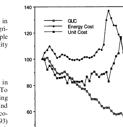
Fig. 1. Generalized unit cost (GUC), energy cost, and Barnett and Morse unit cost for US agriculture. All indicators are indexed to 100 in 1948. Indicators defined in the text. 5.2. Econometric models and tests
This section tests whether the neoclassical model of energy cost in Eq. (8) fits the data. Note that the biophysical model (Eq. (14)) cannot be estimated as it is unidentified. There are several different augmentation trends to estimate but only one equation with which to do so. A typical assumption about the technical change trends Ai
is that they could be second order integrated (I(2)) stochastic processes (Harvey and Marshall, 1991). An I(2) process is a random walk which has a drift term that is itself a random walk. I(2) processes cannot be estimated using a linear re-gression based on Eq. (8) as their first differences are random walks. However, it is possible that the different trends CI(2,1) cointegrate into an I(1) process whose first difference is a constant and a stationary (I(0)) noise process. In this case the drift term can be estimated by including a con-stant in the regression. If the individual technical change trends areI(1) processes then a model that includes the revenue shares of each input as re-gressors can be estimated. Such a model was estimated, but the estimates of these coefficients
Table 1
Energy intensities of inputsa
Mean Standard deviation s/Mean 0.273 31 904
116 958 Capital
45 256
Labor 9055 0.200
Energy 671 711 131 166 0.195 84 654
Fertilizer 301 037 0.281
206 371 33 285
Pesticide 0.161
30 485 5712 0.187
Other
aEnergy Intensities in BTU per 1990 dollar value using the GDP deflator.
were all very large in absolute value (10s or 100s% per year) and so this model was rejected.
Three models are estimated. In all the models the technical change trend is represented by a constant, the other variables are the changes in the logarithms of the relevant variables. The first model estimates Eq. (8) with no restrictions or modifications. The output elasticities are esti-mated as constant regression parameters. The conditionUE=UGis tested by the exclusion of all
the relevant terms. This ‘non-substitutability test’ is the closest that can be got to a test of whether Eq. (14) might fit the data. If the null hypothesis is accepted then energy cost is a function of only the state of technology, the resource stock, and the uncontrolled inputs. The other two models assume that there is substitutability. The second model allows a test of whether the relevant output elasticities are proportional to shares of embodied energy. If the restrictions can be accepted, then despite the presence of substitutability energy cost can still be an accurate indicator of resource quality. The third model is used to test whether price-taking profit-maximization holds and mar-ginal products are proportional to prices. If the restrictions are accepted then generalized unit cost calculated using revenue shares will accurately measure resource quality.
5.2.1. Model 1
DlnU
Et= −a0−SaiDlnXit−aEDlnEt
−Sa
jDlnNjt−aRDlnRt
+aTDlnTt+yt (8a)
The non-substitutability test sets all parameters excepta0,aR, and theajto zero and computes an
F-statistic to test whether the resulting increase in the error sum of squares is statistically significant. If the input – output model is correct, changes in quantities of inputs and total energy use should not be expected to have a systematic effect on energy cost.
5.2.2. Model 2
This model is the same as Model 1 except that the energy and other non-resource inputs elastic-ities are replaced with the relevant share of
em-bodied energy multiplied by the returns to scale described in association with Eqs. (10) and (11):
DlnU
Et= −b0−SbioitDlnXit−bEoEtDlnEt
−SbjDlnN
jt−bRDlnRt+bTDlnTt
+6t (8b)
whereoiandoEare the RHS of Eqs. (10) and (11).
Then a direct test of Eqs. (10) and (11) sets
bi=bE=bT=1 and again the F-statistic for the
restriction is computed. If the restriction is re-jected then energy cost may give misleading indi-cations of changes in resource quality as marginal products are not proportional to embodied energy.
5.2.3. Model 3
In this model the elasticities are replaced with the relevant revenue share:
DlnUEt= −g0−SgiSitDlnXit−gESEtDlnEt
−SgjDlnNjt−gRSRtDlnRt
+gTDlnTt+v (8c)
The coefficients are tested to see whether gi,gE,
gR, andgTare equal to unity — a test of whether
price-taking profit-maximization is an accurate assumption.
Cost is calculated as the sum of the costs of all inputs apart from land, capital, and self labor. To calculate the revenue shares of land, capital, and self labor their shares in factor services as esti-mated by Ball et al. (1995) are found first. Then these shares are multiplied by the share of profit in revenue as proposed by Berndt et al. (1993). Returns to scale for Model 2 are computed by deducting the revenue share of land from unity. The models are estimated using OLS.
5.3. Econometric results
All three models fit the data well both in terms of the adjusted R2 and the Durbin – Watson and
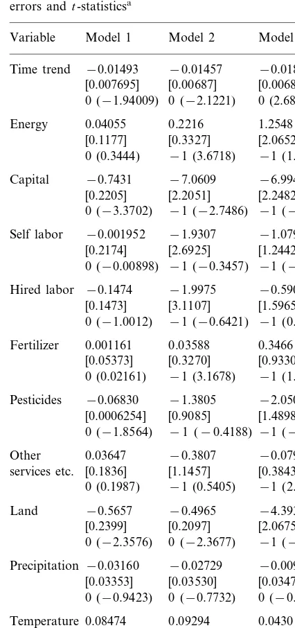
that the aggregate trend is at mostI(1) so that its first difference is stationary. The coefficients and individualt-statistics are presented in Table 3. The coefficients have the expected sign with the excep-tion of energy, fertilizer, and temperature in all three models and other services in Model 1. All the incorrectly signed coefficients are insignificantly different from zero.
The time trend has about the expected magnitude in all three models. The index number based growth rate of multi-factor productivity was about 1.7% p.a. over this period. The econometric estimates are 1.5, 1.5, and 1.8% for the three models, respectively. The mean rate of change in energy cost is 1.0%. So the time trend does track generalized unit cost while the other variables explain the deviation of energy cost from generalized unit cost.
The coefficient on total energy is not significantly different from unity in Models 2 and 3 as expected but is significantly different from unity at the 5% level in Model 1. In Model 1 the coefficient on total energy under the substitutability hypothesis is ex-pected to be one and zero under the non-substi-tutability hypothesis. Many of the other regression coefficients in the three models are not significantly different to zero.
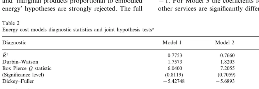
The results of the three joint hypothesis tests are presented in Table 2. Both the non-substitutability and ‘marginal products proportional to embodied energy’ hypotheses are strongly rejected. The full
neoclassical price-taking profit-maximization is also rejected at the 5% level. But at a 3.5% level the neoclassical model would be accepted. So, while neither the energy analysis model nor the strong neoclassical model fits the data very well, the neoclassical model may diverge less from reality.
The individual t-statistics in Table 3 allow an investigation of which variables may be most important in causing the rejection of the restric-tions. For Model 1 the t-statistics for capital and total energy (−3.37 and 8.47) show that their coefficients diverge very significantly from their expected values (zero in both cases) under the null. The coefficient for pesticides is significant at the 10% level. Total energy is probably most important in causing the restrictions to be rejected. For Model 2 the coefficients for capital, energy, and fertilizer all diverge significantly from their expected values under the restrictions. Energy and fertilizer are the most energy intensive inputs (Table 1) and, as expected, their coefficients are greater than−1 and in fact positive. Capital has a coefficient that is significantly less than−1 as expected for a less energy intensive input. However, this pattern is not very clearcut. Both labor inputs have coefficients of less than−1 but not significantly so and other services — the least energy intensive inputs — in fact have a coefficient insignificantly greater than
−1. For Model 3 the coefficients for capital and other services are significantly different from −1
Table 2
Energy cost models diagnostic statistics and joint hypothesis testsa
Model 1 Model 2
Diagnostic Model 3
R( 2 0.7753 0.7660 0.7595
1.7573
Durbin–Watson 1.8203 1.7619
Box PierceQstatistic 6.0400 7.2055 7.3808
(0.6891)
(Significance level) (0.8119) (0.7059)
−5.42748 −5.6893
Dickey–Fuller −5.4166
Joint hypothesis test
16.6266 Nonsubstitutability
(0.0000)
Marginal products proportional to embodied energy 5.9408 (0.0002)
2.4281 Price-taking profit-maximization
at the 5% level and the coefficient of land is different from −1 at close to the 10% significance level. The ex post rents of the two non-labor primary factors — capital and land — diverge substantially from the estimates of Ball et al. (1995) of their ex ante factor services. Therefore, divergence of the coefficients from the shares of ex post rents in revenue is not surprising.
5.4. Time paths of the indicators
Fig. 1 presents three different ‘classical’ (Cleve-land and Stern, 1999) scarcity indicators: general-ized unit cost (UG), energy cost (UE), and Barnett
and Morse’s unit cost (UB).UBis calculated with
value added as the output and capital and labor as inputs. Data sources are described above. An increase in any of the indices indicates an increase in scarcity. The GUC indicator almost forms a lower envelope for the other indicators. Both UE
andUBshow large movements in both directions.
From about 1948 to 1973 both UE andUBare
fairly stable, reaching a minimum in the mid 1960s and rising slightly thereafter. This was a period of falling real energy prices and energy was substituted for capital and labor. UBrises steeply
from 1975 on. The capital stock continued to increase with apparently decreasing returns until 1983 from whence it declined sharply (Fig. 2). Value added rose slowly and became more volatile. The peak in UB in 1983 occurs when the
peak in the capital stock coincides with poor weather.
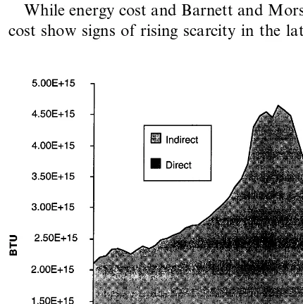
Energy cost also moves up steeply through 1973, peaking in 1975 because direct energy use increased despite rising prices (Fig. 3). Indirect energy use also rose. The apparent reason for this behavior is that output prices rose sharply in 1972 – 1974 as part of the global commodity price boom. The increase in crop prices was bigger than that in energy. Farmers rushed to buy capital and use intermediate inputs in order to increase pro-duction. High energy prices began to have an impact from 1976 onwards. Energy use leveled out and from the second oil shock in 1979 it declined sharply. Crop and livestock output con-tinued to increase at about the same rate as previously. Since 1982 output has fluctuated
Table 3
Energy cost models: regression coefficient estimates, standard errors andt-statisticsa
Model 1 Model 2
Variable Model 3
−0.01493
Time trend −0.01457 −0.01825 [0.006801] [0.00687]
[0.007695]
0 (2.6831) 0 (−1.94009) 0 (−2.1221)
0.04055
Energy 0.2216 1.2548
[0.1177] [0.3327] [2.0652] −1 (1.0918) 0 (0.3444) −1 (3.6718)
−0.7431 −7.0609 −6.9949 Capital
[2.2051] [2.2482] [0.2205]
−1 (−2.6665) 0 (−3.3702) −1 (−2.7486)
−0.001952 −1.9307 −1.0793 Self labor
[0.2174] [2.6925] [1.2442] −1 (−0.06374) 0 (−0.00898) −1 (−0.3457)
−0.1474
Hired labor −1.9975 −0.5906
[3.1107] [1.5965] [0.1473]
0 (−1.0012) −1 (−0.6421) −1 (0.2564) 0.001161
Fertilizer 0.03588 0.3466
[0.05373] [0.3270] [0.9330] −1 (1.4433) 0 (0.02161) −1 (3.1678)
−0.06830
Pesticides −1.3805 −2.0509
[0.0006254] [0.9085] [1.4898] 0 (−1.8564) −1 (−0.4188) −1 (−0.7054) Other 0.03647 −0.3807 −0.07971
[0.1836]
services etc. [1.1457] [0.3843] 0 (0.1987) −1 (0.5405) −1 (2.3947) −0.5657
Land −0.4965 −4.3938
[0.2399] [0.2097] [2.0675] 0 (−2.3576) 0 (−2.3677) −1 (−1.6415) −0.03160
Precipitation −0.02729 −0.009413 [0.03353] [0.03530] [0.03479]
0 (−0.2706) 0 (−0.9423) 0 (−0.7732)
Temperature 0.08474 0.09294 0.04301 [0.2229] [0.2317] [0.2291] 0 (0.3801) 0 (0.4012) 0 (0.1877) 1.3114
Total energy 1.2363 1.2325 [0.1549] [0.1498] [0.1627] 0 (8.4666) 1 (1.5774) 1 (1.4290) 1 (2.0103)
Fig. 2. Output, real value added, and capital stock in US agriculture. All indicators indexed to 100 in 1948.
and 1970s, GUC does not. Similar results have been found by other studies. Researchers who made projections on the basis of the energy cost trend at the time (e.g. Gever et al., 1986) have been shown to have been overly pessimistic (Cleveland, 1995b).
6. Conclusions
In this paper, the use of energy cost as an indicator of natural resource quality and availability has been examined. It was argued that a biophysical theory of value formation needs to account for the use of knowledge in the creation of economic value and should not limit itself to the role of energy alone. It was demonstrated mathematically that energy costs can give false indications of changes in scarcity if substitution between inputs is possible and prices are not proportional to embodied energy. When less en-ergy intensive inputs are substituted for more energy intensive inputs, energy costs will tend to decline, and vice versa.
Statistical tests show that the model of energy cost derived under the neoclassical assumption of smooth differentiability of the production func-tion fits the data reasonably well. Changes in several of the input quantities terms in this model have significant effects on energy cost. If the input – output energy analysis model is correct then these effects should be insignificant. How-ever, the strong neoclassical assumptions of price-taking profit-maximization can be rejected at a 5% level of significance. But at a 3.5% level of significance the full neoclassical model cannot be rejected. Even with substitutability, energy costs could be a good indicator if prices are propor-tional to embodied energy. This hypothesis is also rejected at the highest levels of significance. So while the strong neoclassical model does not fit the data very well, it fits better than the energy analysis model.
There are two possible explanations for this. The neoclassical ecological economics hypothesis is that the factors also contain embodied knowl-edge which cannot be accounted for purely in terms of the energy used to acquire and maintain through the remainder of the 1980s and only
increased above the 1982 level after 1990 (Fig. 2). While energy cost and Barnett and Morse’s unit cost show signs of rising scarcity in the late 1960s
that knowledge and embody it into the factors of production. The second alternative is that the system boundary used to calculate embodied en-ergy is wrong. For example, the enen-ergy cost of labor used in producing non-labor inputs was omitted. Because of these errors, factors of pro-duction may appear to have an effect on energy cost which would disappear with correct measure-ment so that the non-substitution hypothesis could be accepted (Model 1). Alternatively there may be substitutability but correct measures of embodied energy may be proportional to mar-ginal products (Model 2). It is not clear, a priori, if better measurement would improve the perfor-mance of the energy cost indicator. In any case, the energy cost indicator presented in this paper is more comprehensive than some others in the liter-ature. So the problems identified here will likely apply to other calculations of energy cost whichever theory of production is actually cor-rect. Previous efforts (e.g. Cleveland, 1995b; Gever et al., 1986; Hall et al., 1986) to compute energy cost or energy return on investment in US agriculture yield similar time paths.
The generalized unit cost indicator in Eq. (3) would be preferable for measuring those aspects of resource scarcity which energy cost is intended to measure. Empirical calculation of the indicator using index numbers depends on the price-taking profit-maximization assumption. Possible viola-tion of this assumpviola-tion as indicated by the statisti-cal results in this paper should be taken into account. However, violation of the assumption could be due to deficiencies in the rent data in this database. The calculated time series for GUC in US agriculture (Fig. 1) does not show the fluctua-tions in response to economic events that are shown by the other indicators and so seems less problematic than the alternatives. The estimated time trend in all three regression models is closer to the rate of change in GUC than to the rate of change of the other two indicators.
Acknowledgements
I thank Cutler Cleveland, Mick Common, Robert Costanza, and Robert Herendeen for
use-ful comments and discussions which have greatly improved the paper. I also thank V. Eldon Ball and Cutler Cleveland for providing most of the data.
References
Ball, V.E., Bureau, J.-C., Nehring, R., Somwaru, A., 1995. Agricultural Productivity Revisited. United States Depart-ment of Agriculture, Washington DC.
Barnett, H., Morse, C., 1963. Scarcity and Growth: The Economics of Natural Resource Availability. Johns Hop-kins University Press, Baltimore MD.
Berndt, E.R., 1978. Aggregate energy, efficiency, and produc-tivity measurement. Annu. Rev. Energy 3, 225 – 273. Berndt, E.R., Kolstad, C., Lee, J.K., 1993. Measuring the
energy efficiency and productivity impacts of embodied technical change. Energy J. 14, 33 – 55.
Berndt, E.R., Wood, D.O., 1975. Technology, prices and the derived demand for energy. Rev. Econ. Stat. 57, 259 – 268. Brown, M.T., Herendeen, R.A., 1996. Embodied energy analy-sis and emergy analyanaly-sis: a comparative view. Ecol. Econ. 19, 219 – 236.
Chapman, P., Roberts, F., 1983. Metal Resources and Energy. Butterworths, London.
Chen, X., 1994. Substitution of information for energy: con-ceptual background, realities and limits. Energy Policy 22, 15 – 28.
Cleveland, C.J., 1991. Natural resource scarcity and economic growth revisited: Economic and biophysical perspectives. In: Costanza, R. (Ed.), Ecological Economics: The Science and Management of Sustainability. Columbia University Press, New York.
Cleveland, C.J., 1992. Energy quality and energy surplus in the extraction of fossil fuels in the US. Ecol. Econ. 6, 139 – 162. Cleveland, C.J., 1995a. The direct and indirect use of fossil fuels and electricity in US agriculture, 1910 to 1990. Agric. Ecosyst. Environ. 55, 111 – 121.
Cleveland, C.J., 1995b. Resource degradation, technical change, and the productivity of energy use in US agricul-ture. Ecol. Econ. 13, 185 – 201.
Cleveland, C.J., Costanza, R., Hall, C.A.S., Kaufmann, R.K., 1984. Energy and the U.S. economy: a biophysical perspec-tive. Science 225, 890 – 897.
Cleveland, C.J., Stern, D.I., 1993. Productive and exchange scarcity: an empirical analysis of the US forest products industry. Can. J. For. Res. 23, 1537 – 1549.
Cleveland, C.J., Stern, D.I., 1999. Indicators of natural re-source scarcity: a review and synthesis. In: van den Bergh, J.C.J.M. (Ed.), Handbook of Environmental and Resource Economics. Edward Elgar, Cheltenham.
Common, M.S., 1995. Sustainability and Policy: Limits to Economics. Cambridge University Press, Melbourne. Cook, E.F., 1976. Limits to the exploitation of non-renewable
Costanza, R., 1980. Embodied energy and economic valuation. Science 210, 1219 – 1224.
Gever, J., Kaufmann, R.K., Skole, D., Vo¨ro¨smarty, C., 1986. Beyond Oil: The Threat to Food and Fuel in the Coming Decades. Ballinger, Cambridge, MA.
Hall, C.A.S., Cleveland, C.J., Kaufmann, R.K., 1986. Energy and Resource Quality: The Ecology of the Economic Pro-cess. Wiley Interscience, New York.
Hannon, B., 1973a. The structure of the ecosystem. J. Theoret. Biol. 41, 535 – 546.
Hannon, B., 1973b. An energy standard of value. Ann. Am. Acad. 410, 139 – 153.
Harvey, A.C., Marshall, P., 1991. Inter-fuel substitution, tech-nical change and the demand for energy in the UK econ-omy. Appl. Econ. 23, 1077 – 1086.
Kaufmann, R.K., 1987. Biophysical and marxist economics: learning from each other. Ecol. Model. 38, 91 – 105. Kaufmann, R.K., Cleveland, C.J., 1991. Policies to increase
US oil production: Likely to fail, damage the economy, and damage the environment. Annu. Rev. Energy 16, 379 – 400.
Mas-Colell, A., Whinston, M.D., Green, J.R., 1995. Microeco-nomic Theory. Oxford University Press, New York.
O’Connor, M.P., 1993. Entropic irreversibility and uncon-trolled technological change in the economy and environ-ment. J. Evol. Econ. 3, 285 – 315.
Perrings, C.A., 1987. Economy and Environment: A Theoreti-cal Essay on the Interdependence of Economic and Envi-ronmental Systems. Cambridge University Press, Cambridge.
Ruth, M., 1995. Information, order and knowledge in eco-nomic and ecological systems: implications for material and energy use. Ecol. Econ. 13, 99 – 114.
Spreng, D., 1993. Possibilities for substitution between energy, time and information. Energy Policy 21, 13 – 23.
Stern, D.I., 1994. Natural Resources as Factors of Production: Three Empirical Studies. Ph.D. Dissertation, Department of Geography, Boston University, Boston MA.
Stern, D.I., 1997. Limits to substitution and irreversibility in production and consumption: a neoclassical interpretation of ecological economics. Ecol. Econ. 21, 197 – 215. US Department of Commerce, Bureau of Economic Analysis,
1986. National Income and Product Accounts 1929 – 1982. United States Government Printing Office, Washington DC.
US Department of Commerce, Bureau of Economic Analysis, various issues. Survey of Current Business. United States Government Printing Office, Washington DC.
![The significance of mycorrhiza in regeneration of merbau [Intsia bijuga (Colebr.) O. Kuntze] originating from Papua](data:image/gif;base64,R0lGODlhAQABAIAAAP///wAAACH5BAEAAAAALAAAAAABAAEAAAICRAEAOw==)