SOME CHARACTERISTICS OF ATMOSPHERIC BOUNDARY LAYER OVER
MAKASSAR
Alimuddin Hamzah Assegaf1*, Wasir Samad2, Sakka1
Submitted: 14 January 2018 Accepted: 19 February 2018
ABSTRACT.
Some upper air atmospheric parameters measured during period of 2011-2016 by means of radiosonde located at Hasanuddin International Airport were examined for characterization of boundary layer over Makassar, Indonesia. These data, combined with surface atmospheric parameters were used to calculate some boundary layer parameters using AERMET model which based on Monin-Obukhov similarity theory. The obtained Monin-Obukhov length which reflecting atmospheric stability then converted into traditional Pasquill-Gifford stability classification. Examination of wind characteristics of wind showing clearly their dependence of the day, season and height. Winds dominantly flows from the southeast during the daytime with the relatively larger velocity and from the northwest with smaller velocity during the nighttime. Interpretation of monin-obukhov length using Pasquill-Gifford stability classification showing that the atmosphere was dominantly unstable during the daytime and dominantly stable during the nighttime. These atmospheric stabilities were also varied during seasons. The height of convective boundary layer (CBL) was start to rise in the morning and reaching its maximum in the afternoon (18:00) at the mean value of 2 km. Meanwhile, the height of mechanical boundary layer (MBL) during the day time forming parabolic curve with its maximum value of 1.2 km at noon. These indicated that any released pollution from the stack will be less dispersed during the nighttime due to the fact of lower mixing height, lower wind speed, atmosphere become more stable, and it dispersed in different direction compare to the daytime.
Keywords: atmospheric boundary layer, atmospheric stability, AERMET, boundary layer height
INTRODUCTION
Study on atmospheric boundary layer plays important role in air quality modelling. Information about mixing height, atmospheric stability, wind profile, and turbulence characteristics will be valuable on predicting the behaviour of air pollutant dispersion. The wind will determine the direction and the speed of pollutant away from its source. The atmospheric turbulence will determine the turbulence dispersion. The temperature affects the rise of a buoyant plume 00 2017; 0).
Preparation of meteorological data for air quality modelling is one of important step, that challenging for development country, such as Indonesia. The data can be obtained from satellite, global model, or surface station. Satellite can cover the whole globe, but its resolution is too coarse to be used in short range model. Other choice is to use the global meteorological model, such as MM5 or WRF 0;0; 0; 0). We start from the coarse grid, then downscaling at the area of interest. Preparation of the model for generating long term prediction (in the order of 5 years or more) required huge computer resource and some detail of parameters setting need advance expertise. The best data is from the measurement at local surface station. Unfortunately, the availability of surface meteorological station, that provide upper air meteorological profile data is very few in the
*Alimuddin Hamzah Assegaf
1
Department of Physiscs, Hasanuddin University
2
Departmen of Marine Science, Hasanuddin University Jl. Perintis Kemerdekaan Km.10, Makassar 90245, Indonesia Email: [email protected]
development country, such as Indonesia. Until recently, some major airports in Indonesia are equipped with radiosonde to measure the meteorological profile around the airport.
This paper describes the preparation of meteorological data based on the local station. Both surface and upper meteorological data were processed to obtain boundary layer parameters such as sensible heat flux, friction velocity, convective velocity scale, boundary layer height, as well as Monin-Obukhov length (L) 0).
MATERIALS AND METHODS
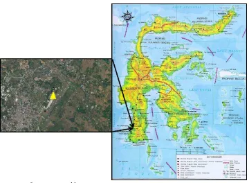
Location and Data Preparation
Figure 1. Location map of Sultan Hasanuddin International Airport (inset on map)
AERMET Model
The AERMET model is a meteorological processor for the AERMOD model 0; 0, together with AERSURFACE model (as a terrain/morphology processor) 0; 0. AERMOD system is regulated model in USA, Canada, and some European countries. It utilizes the principle of surface heat equilibrium to calculate friction velocity, convective velocity scale, as well as Monin-Obukhov length (L) 0 and determine whether the atmosphere is stable or unstable. Planetary boundary layer (PBL) is divided into two types: convective boundary layer (CBL) and stable boundary layer (SBL). CBL is developed during the day. It is driving by surface heating and can cause moderate to strong vertical mixing 0. Meanwhile, SBL develops at night, driven by surface cooling and causing little to no vertical mixing. In calculating the transfer of surface heat to the atmosphere and vice versa, AERMET refers to the formula proposed 0;0; 0, which calculated the solar radiation flux as a function of temperature, cloud cover and angle of the sun. Further more sensible heat flux is calculated as a function of solar radiation flux and Bowen ratio. Monin-Obukhov length will be calculated iteratively based on convective velocity scale information, temperature and wind speed. Next steps are calculating the stability of the atmosphere and
the thickness of the boundary layer (convective and mechanical boundary layers). The AERMET
convention is used as follows: day time period is 07:00~18:00 (CBL period) and night time period is 18:00~07:00 LST (SBL period). 07:00 is the transition between SBL and CBL; vice versa 19:00 is the transition between CBL and SBL. The result of AERMET is processed further to have quarterly quantity (25%, 50% and 75% percentile) of the processed results.
RESULTS AND DISCUSSION
Wind Roses and Upper Air Profile
(a)
(b)
(c)
Figure 2. Wind roses of the daily variation (a) day time (b) night time, and (c) day-night during period 2011-2016
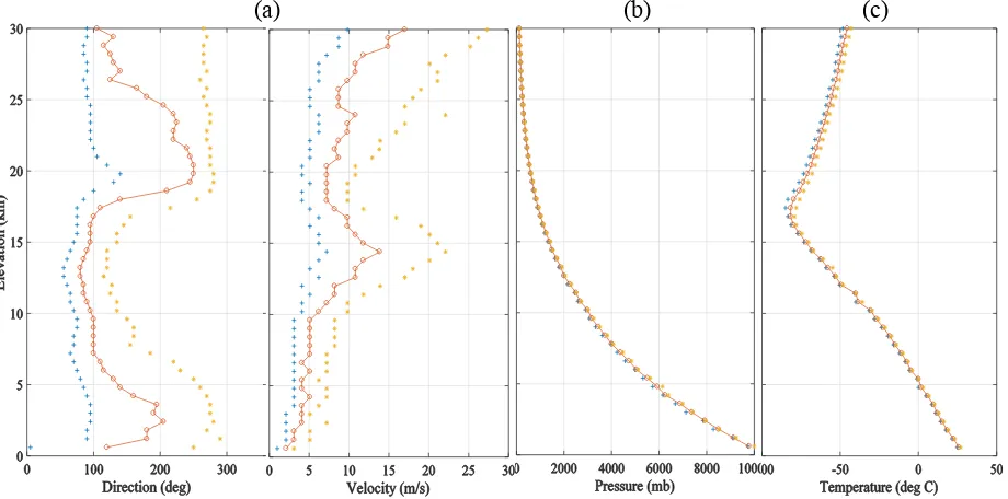
(a)
(b) (c)
Figure 3. Upper air profile: (a) Wind velocity and dicrection, (b) pressure, (c) temperature
Sensible Heat Lux
The sensible heat flux is the energy flux from the atmosphere to the ground driven by temperature differences between the ground and the atmosphere. It is the energy flux transferred from or to the ground. During the daytime, energy radiates from the ground into the atmospheric boundary layer, while during the night the boundary layer supplies energy to the ground.
(291.8 Watt/m2). There is a little variation over the month, where it has maximum on October and
minimum on June (Figure-4b) and overall median is 186.mm Watt/m2
Figure-4. Variation of sensible heat flux Daily (left panel), Monthly (right panel)
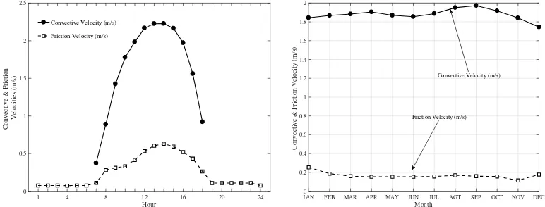
Convective and Friction Velocities 2.36 m/s. The curve path is following the sensible heat flux as the energy supply for the turbulence dynamic. Air flowing over a surface exerts a shear stress that
depends on the level of turbulence in the boundary layer. Turbulence in the stable boundary layer is generated by wind shear, and inhibited by the stable potential temperature gradient. Observations indicate that the height of the boundary layer, which is the height to which the turbulence extends, is related to the surface friction velocity. The maximum friction velocity is 0.73 m/s with range of 0.69 m/s, and overall median is 0.15 m/s. Figure 5 (right panel) shows that the maximum convective velocity is 2.29 m/s which occur on September. Small variation (0.1 m/s) of friction velocity which is has median of 0.88 m/s. The surface friction velocity, u*, is a measure of mechanical turbulence and is directly related to the surface roughness.
Figure 5. Variation of convective and friction velocities of daily (left panel) and monthly (right panel)
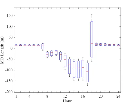
Monin-Obukhov Length
Monin-Obukhov (MO) length reflects the stability of the atmosphere. When MO length (Figure 6) is negative, it indicates unstable conditions (positive surface temperature flux), infinite at neutral, and positive under stable conditions. Instability arises in the morning and tends to increase as more heat accumulated in the day time. It reached its maximum in the afternoon, just before transition time. When the
MO length is converted into Pasquill-Gilford (PG) stability criteria (see Table 1), information on atmospheric stability distribution can be more explore. During the night time, the atmospheric stability is dominated by class G (moderately stable) and following by class H (very stable). On the contrary, the atmospheric condition is very unstable (class A) during the day time. Small variations are over the months, but mostly very stable (during the night time) and very
JAN FEB MAR APR MAY JUN JUL AGT SEP OCT NOV DEC
Month
.
Table 1. Conversion of MO length into PG stability criteria 0
Stability Class MO Length (m)
A: very unstable -40 L < -12
Figure 7. Atmospheric stability distribution over day and month
Height of Boundary Layers
The rapid boundary layer growth in the morning starting at 7 to 15 LST and tends to slow at 16~18 LST. It reflects contribution of turbulence to push up the boundary layer ceiling and ended at dissipation due to decrease of solar heat in the afternoon. The maximum height of CBL is 1.9 km at 17 LST. The MBL is also growth in the period of 7~13 LST and has maximum 1.2 km at 14 LST and finally decreases.
MBL is strongly influenced by wind friction. As shown in Figure 8 (left panel), the height of CBL and MBL is about 1.3~1.5 km and 0.4~0.7 km, respectively. High boundary layer episodes typically occur in the period of August ~ October. It is coincidence with dry air due to strong sensible heat which can be seen in Figure-4 and Figure-8 (right
panel).
Figure 8. Variation of ABL height of daily (left panel) and monthly (right panel)
1 4 8 12 16 20 24
CONCLUSION
The following conclusion can be drawn from the discussion: The wind dominantly blows from South-Southeast (SSE) in the day time and from North in the night time with lower speed. The convective and friction velocity is about 1.9 m/s and 0.2 m/s, respectively. The height of CBL and MBL is about 1.5 km and 0.5 km, respectively
REFERENCES
Assegaf, AH. and Jayadipraja EA, Modeling of CO Dispersion from Tonasa Cement Factory Stack Using AERMOD Model, in Physics National Seminar: Makassar 2015, Makassar, Indonesia, Faculty of Mathematics and Natural Sciences, Hasanuddin University, (2015) (in Bahasa Indonesia).
Cimorelli, A. J, Steven G.Perry, Akula Venkatram, Jeffrey C.Weil, Robert J.Paine, Robert B.Wilson, Russell F.Lee, Warren D.Peters, Roger W.Brode, 2005: AERMOD: A Dispersion Model for Industrial Source Application. Part I: General Model Formulation and Boundary Layer Characterization, Journal
of Applied Meteorology 44, 682-693.
Grell, G. A., J. Dudhia and D. R. Stauffer, 1994: A Description of the fifth generation Penn State/ NCAR mesoscale model (MM5), NCAR Tech
Note, NCAR/TN-398+STR, 117
Holtslag A.A.M. and van Ulden A.P. (1983). A simple scheme for daytime estimates of the surface fluxes from routine weather data. J. Clim. Appl.
Meteorol. 22, 517–529.
Holtslag A.A.M. and de Bruin H.A.R. (1988). Applied Modeling of the Nighttime Surface Energy Balance over Land. J. Appl. Meteorol. 27, 689– 704.
Jayadipraja EA, Daud A, Assegaf AH, Maming. Applying Spatial Analysis Tools in Public Health: The Use of AERMOD in Modeling the Emission Dispersion of SO2 and NO2 to
Identify Exposed Area to Health Risks. Public Health of Indonesia 2016;2(1): 20-27
Jesse L. Thé, Russell Lee, Roger W. Brode (2011): Worldwide Data Quality Effects on PBL Short-Range Regulatory Air Dispersion Models, Weblakes Environment Consultants Inc.
Monin, A.S. and A.M. Obukhov (1954): Basic laws of turbulent mixing in the surface layer of the atmosphere (English translation by John Miller for Geophysics Research Directorate, AF Cambridge Research Centre, Cambridge, Massachusetts, by the American Meteorological Society), Originally published in Tr. Akad. Nauk SSSR Geophiz. Inst. 24(151):163-187
Perry, S. G. et. al., 2005: AERMOD: A Dispersion Model for Industrial Source Application. Part II: Model Performance against 17 Field Study Databases, Journal of Applied Meteorology 44, 696-708.
Pelliccioni, A., P. Monti, C. Gariazzo, and G. Leuzzi.
“Some Characteristics of Urban Boundary
Layer Above Rome, Italy, and Applicability of Monin-Obukhov Similarity.” Environ Fluid Mechanics 12 (2012): 405-428
Stull, Roland B., 1988; An Introduction to boundary layer meteorology. Published by Kluwer Academic Publishers. The Netherlands.
Stull, Roland B., 2017; Practical Meteorology: An Algebra-based Survey of Atmospheric Science. Department of Earth, Ocean and Atmospheric Sciences. University of British Colombia. Vancouver Canada.
US Environmental Protection Agency, 1998a: AERMOD: Revised Draft – User’s Guide for the AMS/EPA Regulatory Model – AERMOD. Office of Air Quality Planning and Standards, Research Triangle Park, NC
US Environmental Protection Agency, 1998b: Revised Draft – User’s Guide to the AERMOD Terrain Preprocessor (AERMAP). Office of Air Quality Planning and Standards, Research Triangle Park, NC.
Van Ulden A.P. and Holtslag A.A.M. (1985). Estimation of atmospheric boundary layer parameters for diffusion applications. J.