Dynamic Threshold Based Load Balancing Algorithms
Neeraj Rathore1
Springer Science+Business Media New York 2016
Abstract In this scenario, dynamic and decentralized Load Balancing (LB) considers all the factors pertaining to the characteristics of the Grid computing environment. Dynamic load-balancing algorithms attempt to use the run-time state information to make more informative decisions in sharing the system load and in decentralization, algorithm is executed by all nodes in the system and the responsibility of LB is shared among all the nodes in the same pool. For this purpose, in this work, an extensive survey of the existing LB has been done. A detailed classification and gap analysis of the existing techniques is presented based on different parameters. The issue of LB in a Grid has been addressed while maintaining the resource utilization and response time for dynamic and decentralized Grid environment. Here, a hierarchical LB technique has been analyzed based on variable threshold value. The load is divided into different categories, like, lightly loaded, under-lightly loaded, overloaded, and normally loaded. A threshold value, which can be found out using load deviation, is responsible for transferring the task and flow of workload information. In order to improve response time and to increase throughput of the Grid, a random policy has been introduced to reduce the resource allocation capacity etc. Poisson process has been used for random job arrival and then load calculation has been done for assigning job to the appropriate Processing Entity for balancing the load in the pool. After balancing the load, it comes into the normally loaded pool, and then Job Migration process is executed. The performance of the proposed model, algorithms and techniques has been examined over the GridSim simulator using various parameters, such as response time, resource allocation efficiency, etc. Experimental results prove the superiority of the pro-posed techniques over the existing techniques.
Keywords Grid computingGridSimArchitectureLoad balancingWorkload Job Migration
& Neeraj Rathore
[email protected]; [email protected] 1
Department of Computer Science and Engineering, Jaypee University of Engineering and Technology, Guna, M.P., India
1 Introduction
Grid computing has recently become one of the most important research topics in the field of computing. The Grid paradigm has gained popularity due to its capability to offer easier access to geographically distributed resources operating across multiple administrative domains. The grid environment is considered as a combination of dynamic, heterogeneous and shared resources in order to provide faster and reliable access to the Grid resources. For efficient resource management in Grid, the resource overloading must be prevented which can be obtained by proper Load Balancing mechanisms [1–3].
In the existing work, a dynamic, decentralized Load Balancing technique is proposed that considers all the factors pertaining to the characteristics of the Grid computing environment [4]. A dynamic threshold value is used at each level and the value of the threshold is dynamically changing according to the Grid size in the network. A well-designed information exchange scheduling scheme is adopted in the proposed technique to enhance the efficiency of the Load Balancing model. A comparative analysis between the existing technique and proposed exhibits why the proposed technique is better than other existing algorithms. The proposed technique is a new version of the LB mechanism based on random policy. The design of the system environment, LB process for random job arrival through Poisson process has been developed and the flowchart of proposed Hier-archical Load Balancing technique [5–12] along with fitness function has been presented in this paper.
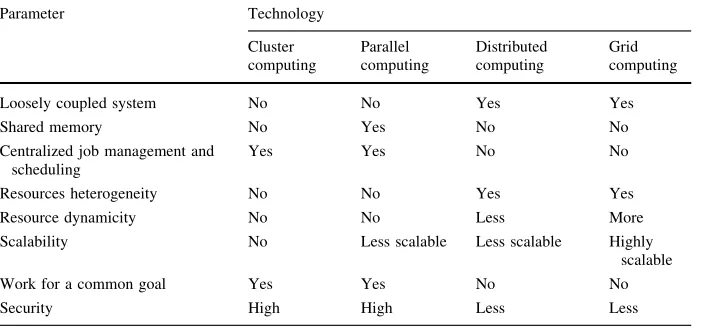
Sharing resources among organizational and institutional boundaries needs an infras-tructure to coordinate resources of boundaries within so called virtual organizations. Grid technology builds the infrastructure for virtual organization. Such infrastructure should offer an easy management of forming virtual organizations, sharing resources, discovering services and consuming services. Grid functionally combines globally distributed com-puters and information systems for creating a universal source of computing power and information. A Grid can offer a resource balancing effect by scheduling and load balancing of Grid jobs at machines with low utilization. A proper load balancing across the Grid can lead to improve overall system performance and a lower turnaround time for individual jobs. This is very crucial concern in distributed environment, to fairly assign jobs to resources [13–16]. Table1shown the different load balancing techniques comparison.
The main goal is to distribute the jobs among processors to maximize throughput, maintain stability, and resource utilization. This is achieved by proper load balancing techniques. Load balancing is done basically to do following benefits.
• Load balancing reduces mean job response time under job transfer overhead. • Load balancing increases the performance of each host.
• Small jobs will not suffer from starvation.
1.1 Our Contribution
Due to the appearance of load balancing challenge in grid computing, there is currently a need for a hierarchical load balancing algorithm which gets into the account grid archi-tecture, heterogeneity, response time, resource allocation and makespan. Taken altogether, the main contributions and novelties of our research work are as follows:
grid computing environment mentioned above. This technique is good for back up and support, in case of server failure.
2. The proposed approach eliminates the scalability complexity of a site. Most of the existing load balancing techniques uses a static threshold value that is somehow good for restricted network size but cause problems in a large scale grid environment. It may lead to scalability and response time issues etc. To overcome existing problems,dynamic threshold valuehas been used in the proposed work. Every time when the application or node has been increased or decrease, threshold value has been calculated. This is easy to use and more supportive with the hierarchical load balancing technique.
3. An efficient load balancing technique is adopted to enhance the efficiency of the load balancing model. We have proposed an extended version of the random policyfor selecting the node during load balancing and initiated by under loaded or overloaded node in the pool of shared nodes.
This section gives an overview of all aspects of Grid Computing. It discusses the tech-nologies like distributed computing, cluster computing etc. and various kinds of Grid based services, various types of Grid, components of Grid and benefits of a Grid environment. In the Sect.2preliminaries has been discussed for the proposed Load Balancing algorithms. Related work is discussed in Sect.3. The Sect.4focuses on the system model, structure of the load balancing model along with the design of the system environment and its appli-cation to the network environment. Then, the problem description, flowchart, fitness functions have been presented for the proposed model. The Load Balancing flowchart and algorithms have been proposed for the model in the Grid environment describes in Sect.5. To understand Load Balancing Technique, a case study has been considered in Sect.6. Performance evaluations and simulation results have been presented in Sect. 7. Finally, Sect.8is dedicated to conclusion and future work.
2 Preliminaries
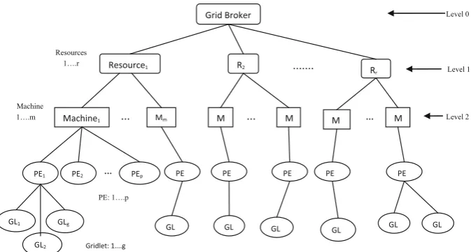
Qureshi and Rehman [16] had documented Grid architecture for Load Balancing, as illus-trated in Fig.1. They have used, Poisson process for random job arrival with a random computation length. Considering that the jobs are sequenced, mutually independent with the Table 1 Difference between technologies
Parameter Technology
Loosely coupled system No No Yes Yes
Shared memory No Yes No No
Centralized job management and scheduling
Yes Yes No No
Resources heterogeneity No No Yes Yes
Resource dynamicity No No Less More
Scalability No Less scalable Less scalable Highly
scalable
Work for a common goal Yes Yes No No
arrival rate and can be executed on any site. Furthermore, the site should meet the jobs demand for the computing resource and the amount of data transmitted. Each processor can only execute one job at a time and execution of a job cannot be interrupted or moved to another process during current execution. This model has been divided into three levels: Level-0 Broker, Level-1 Resource, and Level-2 Machine Level. When a new job known as Gridlet arrives on a machine, it may go to underlightlyloaded, lightly-loaded, overloaded and normal loaded resources by load calculation being computed at each node. In order to compute the mean job response time analysis one Grid Broker (GB) section as a simpli_ed Grid model has been considered. Grid Broker is the top manager of a Grid environment. It is liable for sustaining the overall Grid activities of scheduling and rescheduling. It acquires the infor-mation of the work load from Grid resources and sends the tasks to resources for optimization of load. Resource that comes next to Grid Broker in the hierarchy, are connected through internet. The resource manager is responsible to maintain the scheduling and Load Balancing of its machines and it also sends an event to the Grid broker during overload. The machine is a Processing Entity (PE) manager, responsible for task scheduling and Load Balancing of its PE’s connected with various resources via LAN. PE manager also sends an event to resource during overload. PE’s next to machines are mainly responsible for calculating workload and threshold values for Load Balancing, Job Migration and passes the load information upwards to machines via buses. Gridlet is considered as a load and assigned to any of the PE’s according to their capability (i.e. Computational speed, queue length, etc.).
3 Related Work
traditional distributed systems load balancing policies. Some of them which have been studied are described from next section and some of them are summarized here.
types of strongly influencing system parameters such as the job arrival rate, processing rate, and load on the processor and use this information for estimating the finish time of a job on a buddy processor. The authors address various issues by proposing two job migration algorithms, which are Modified ELISA (MELISA) and Load Balancing on Arrival (LBA). MELISA, which is applicable to large-scale systems is a modified version of ELISA [28] in which consider the job migration cost, resource heterogeneity, and network heterogeneity when load balancing is considered. The LBA algorithm, which is applicable to small-scale systems, performs load balancing by estimating the expected finish time of a job on buddy processors on each job arrival. The paper [29] describes a centralized model for dynamic load balancing with Multiple Supporting Nodes in dis-tributed systems. The objective of this algorithm is to reduce the communication delay and traffic up to some extent, and this is obtained because the load is transferred within the cluster itself (from the primary node to supporting node).
4 System Model and Problem Description
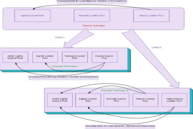
The work, proposed here, is an enhancement of the work [2, 16] discussed above. It suggests the necessity of quantification of the load in order to achieve Load Balancing in computational grid. Quanti_cation of the load is done and the objective function is derived based on the load distribution of the computational nodes. Response time and resource allocation have been recorded as a fair contribution of this research. Furthermore, it extends the existing technique into two cases as discussed in Table2.
Two cases for the proposed technique have been considered. In first case, lightly loaded node is divided into lightly and under lightly loaded categories in the context of variable threshold and standard deviation. Thus, the nodes are divided into four pools. This tech-nique minimizes the searching time to find out the receiver machine in order to transfer the Gridlets. A well-designed information exchange scheduling scheme is adopted in the proposed technique to enhance the efficiency of the Load Balancing model.
In the second case, load is divided lightly loaded into lightly and under lightly loaded categories and heavily loaded node into heavily and highly heavily loaded categories in the context of variable threshold and standard deviation. Thus, here the nodes are divided into five pools. This technique minimizes the searching time (as compared to the existing technique) but increases the ambiguity in the form of comparison that can increase exponentially.
To find an appropriate node for migration is complex task that can enhance the cost and storage capacity as compared to the existing techniques. Therefore, first case is better than existing and second case in all perspectives. Thus, the first case has been implemented in this thesis work. A comparative analysis depicts the difference between all the techniques and exhibits why the proposed algorithm is better than any other existing algorithms presented in Fig.1.
In Grid environments, the shared resources are dynamic in nature, which in turn affects application performance. Workload and resource management are two essential functions provided at the service level of the Grid software infrastructure. To improve the global throughput of these environments, effective and efficient load balancing algorithms are fundamentally important.
Load balancing is the process of redistributing the work load among nodes of the distributed system to improve both resource utilization and job response time while also avoiding a situation where some nodes are heavily loaded while others are idle or doing little work. Static load balancing strategies are not suitable for the environment where resources are heterogeneous and dynamic in nature. In this case dynamic algorithms work well.
A dynamic load balancing algorithm assumes no a priori knowledge about job behavior or the global states of the system, i.e. load balancing decisions are solely based on the current status of the system. Centralized load balancing schemes, the reliance on one central point of balancing control could limit future scalability and not suitable for Grid environment. The distributed scheme helps solve the scalability problems, thus Table 2 Comparison between three techniques
Techniques Existing technique Proposed technique (Case-1) Proposed technique (Case-2)
Categories Divided into three pools like: lightly, normally, heavily
Divided into four pools like: under lightly, lightly, normally,
node has to check all the nodes in the lightly loaded pool
According to load percentage overloaded node is checked into one pool either lightly or under lightly loaded pool on the basis of sorting
Checking has been done in all four pools
Comparisons 1 2 4 (exponential increase)
Scheduling No Yes Yes
Sorting No Yes ascending—under lightly and lightly loaded pool
descending—heavily loaded pool
Yes
Policy Not applicable Random: means process can be executed vice versa also (lightly loaded node can also search heavily loaded node)
Any
Response time
Low High (know about the status of each pool and sorted all nodes in order)
Medium
Throughput Low High (high availability) Medium
Resource allocation capacity
Low High (due to idea of load percentage)
Medium
Cost Low Medium High
Time High (each node has explored in the pool)
development an efficient dynamic distributed load balancing is important to improve the overall performance of Grid.
So to improve overall system performance and to reduce the average job response time and execution time development of an efficient dynamic distributed load balancing tech-nique is very important. The focus of our study is to consider factors which can be used as characteristics for decision making to initiate Load Balancing.
5 Load Balancing Model
Proposed load balancing technique is based on hierarchal model. There are three levels in this hierarchy: Grid-Level, Resource-Level (cluster), and Machine-Level shown in Fig.2. It is assumed that the Grid-Level consists of a collection of Clusters connected by a communication network. Each resource/cluster may contain multiple machines and each machine can have more than one Processing Element. The machines in the resource are heterogeneous in nature. The differences may be in the hardware architecture, operating systems, and processing power. In this study, heterogeneity only refers to the processing power of the machine.
The processing power of the Grid cluster is measured by the average CPU speed across all computing nodes within the machine.
Each level in this hierarchy (illustrated in Fig.2) is explained in detail. Grid Broker is the top manager of a Grid environment which is responsible for maintaining the overall Grid activities of scheduling and rescheduling.
It gets the information of the work load from Grid resources. It sends the tasks to resources for optimization of load. Resource is next to Grid Broker in the hierarchy. It is responsible for maintaining the scheduling and load balancing of its machines. Also, it sends an event to Grid broker if it is overloaded. Machine is a Processing Element (PE) manager. It is responsible for task scheduling and load balancing of its PEs. Also, it sends an event to resource if it is overloaded.
Grid Broker
Level 0: Grid Broker (GB)
This first level has a virtual node called Grid Broker, which is root of hierarchy. Any GB manages a pool of Resource Managers (RMs) in its geographical area. The role of GB is to collect information about the active Machine and PEs managed by its corresponding RMs. GBs are also involved in the task allocation and load balancing process in the Grid. Grid Broker performs the following functions:
• It maintains the workload information of the entire hierarchy.
• It manages a global load balancing between the Grid resources, for this one algorithm is called known as a GB-level load balancing.
• It sends the load balancing decisions to the resources of level-1 for execution.
Level 1: Resource Manager (RM)
Each virtual node of this level, called resource manager, is associated with a physical Grid cluster. Every RM is responsible for managing a pool of Machine. The role of the RM is to collect information about active processing elements in its pool. The collected information mainly includes CPU speed, and other hardware specifications. Also, any RM has the responsibility of allocating the incoming jobs to any processing element in its pool according to a specified load balancing algorithm. The range for the number of RMs is considered as from 1 to r as shown in Fig.5. In our load balancing strategy, this virtual node is responsible for:
• Maintaining the workload information relating to each one of its machines.
• Estimating its associated machines workload, and allocating the incoming jobs to any machine in its pool.
• Managing a local load balancing, for this one algorithm is called this algorithm is named as a Resource-level load balancing.
• Taking decision to invoke GB-level load balancing algorithm.
Level 2: Machine Manager (MM)
At this last level, the processing Element of the Grid has been founded which linked to their respective machines, and these machine linked to their respective resource/cluster.
Any machines can join the Grid system by registering within any RM and offer its computing resources to be used by the Grid users. Each Machine can have more than one PEs and each PEs have some specified CPU speed in terms of Millions Instruction Per Second (MIPS) rating. The ranges for number of MMs in any Resource are considered as from 1 to m. Each machine can have one or more number of PE attached with it and are responsible for actual execution of jobs or Gridlets. Once Gridlet is submitted to Machine, MM will assign this Gridlet to the available PEs. Migration of Gridlet is performing from this level only. The range for number of PEs in any particular Machine is considered as from 1 to p. Each MM is responsible for:
• Maintaining workload information of its associated PEs. • Estimating workload of all PEs.
• Managing a local load balancing, for this one algorithm is called this algorithm is named as Machine-level load balancing.
• Deciding whether to invoke Resource-level load balancing algorithm.
• It gives more preferences to a local task transfer (within a resource or cluster) than global transfer (task transfer between resources or clusters).
• It reduces tasks moving across the Grid broker of a Grid architecture;
• It allows performing more than one load balancing operation at the same time. • It supports Grid heterogeneity and scalability.
• It is totally independent from any physical Grid architecture.
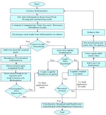
The flowchart of the proposed Load Balancing technique has been shown in Fig.3.
5.1 Proposed Algorithm
Our proposed Load Balancing technique is hierarchal based in heterogeneous Grid envi-ronment. Here heterogeneity in terms of processing capability of each machine. The assumptions has taken that processing capability of each PE is same for single machine. Our proposed algorithm is used sender initiated strategy, which means the machine or resources which want to transfer the Gridlet will search for the under lightly loaded machine or resources.
5.2 Load Balancing Approach
Our proposed load balancing approach works at three levels: Broker, Resource, and Machine Level (Level-0, Level-1, and Level-2 respectively). When a new Gridlets arrives at a machine, it submits it to a PE, which is lightly loaded. Also, after any of the defined four activities will happen, it checks the load of all PEs and classifies them: under lightly loaded, lightly loaded, over loaded, normal.
In our proposed scheme PEs or machines or Resources are categorized into four parts which is under lightly loaded (PE/Machine/Resource), lightly loaded (PE/Machine/Re-source), over loaded (PE/Machine/Re(PE/Machine/Re-source), normal (PE/Machine/Resource). Each of them is described below:
• Normal Loaded Any PE/Machine/Resource comes under this category if its load is equal to some pre-specified threshold value.
• Over loadedAny PE/Machine/Resource comes under this category if its load is greater than some pre-specified threshold value.
Again lightly loaded have been divided into lightly and under lightly loaded, because to minimize the searching time to find out the receiver machine to transfer the Gridlets (need to check only either in under lightly loaded or lightly loaded machines, which reduces the searching time).
• Lightly loaded Any PE/Machine/Resource comes under this category if its load is
[50 % of some pre-specified threshold value.
• Under Lightly loadedAny PE/Machine/Resource comes under this category if its load is\50 % of some pre-specified threshold value.
The proposed load balancing scheme is simulated on the GridSim.
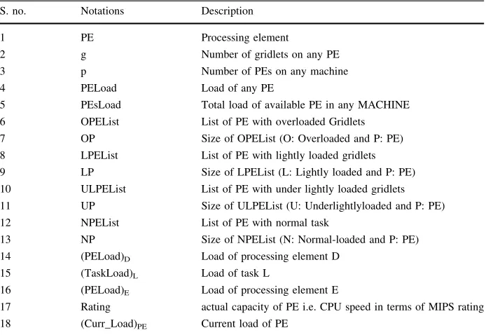
5.3 Notations Used in Algorithms
Notations that are used at PEs level are summarized in Table3. Notations that are used at Machine level are summarized in Table4. Notations that are used at Resource level is summarized in Table5.
5.4 Formulas Used
5.5 Load Parameter
Proposed algorithms have used different load parameter at each level such as PE level load is denoted byq, machine level load is denoted byg, and the resource level load is denoted byqand Load parameter is given in Table7. We have taken this parameter from paper [28].
Table 3 Notations used at PE level
S. no. Notations Description
1 PE Processing element
2 g Number of gridlets on any PE
3 p Number of PEs on any machine
4 PELoad Load of any PE
5 PEsLoad Total load of available PE in any MACHINE 6 OPEList List of PE with overloaded Gridlets
7 OP Size of OPEList (O: Overloaded and P: PE)
8 LPEList List of PE with lightly loaded gridlets 9 LP Size of LPEList (L: Lightly loaded and P: PE) 10 ULPEList List of PE with under lightly loaded gridlets 11 UP Size of ULPEList (U: Underlightlyloaded and P: PE)
12 NPEList List of PE with normal task
13 NP Size of NPEList (N: Normal-loaded and P: PE)
14 (PELoad)D Load of processing element D
15 (TaskLoad)L Load of task L
16 (PELoad)E Load of processing element E
17 Rating actual capacity of PE i.e. CPU speed in terms of MIPS rating 18 (Curr_Load)PE Current load of PE
Table 4 Notations used at machine level
S. no. Notations Description
1 M Number of machines on any resource
2 MLoad Load of any machine
3 MsLoad Total load of machines in any resource
4 OMList List of machine with overloaded PEs
5 OM Size of OMList (O: Overloaded and M: Machine)
6 LMList List of machine with lightly loaded PEs
7 LM Size of LMList (L: Lightlyloaded and M: Machine)
8 ULMList List of machine with under lightly loaded PEs
9 UM Size of ULMList (U: Underlightlyloaded and M: Machine)
10 NMList List of machine with normal PEs
11 NM Size of NMList (N: Normal-loaded and M: Machine)
12 (MLoad)D Load of machine D
Details of these parameters are as follows.
In paper [28], authors use the concept of group and element. Depending on cases, a group designs either a cluster or the Grid (level 1 or level 0 in the tree). An element is a group component (worker node of level 2 or cluster of level 1).
They have considered standard deviation over the workload index, in order to measure the deviation between its involved elements. To consider the heterogeneity between nodes capabilities, they propose to take as workload index the processing time. Processing time of an entity (element or group) is defined as the ratio between workload (LOD) and capability (SPD) of this entity.
They define a balance threshold, denoted asq, from which they said that the standard deviation tends to zero and hence the group is balanced. For this purpose, they propose to define a thresholdq[[0–1]. They have given the following expression: If (rBq) Then the group is Balanced Else it is Imbalanced.
Table 5 Notations used at resource level
S. no. Notations Description
1 r Number of resources
2 ORList List of resource with overloaded machines
3 OR Size of ORList (O: overloaded and R: Resource)
4 LRList Machine with lightly loaded PEs
5 LR Size of LRList (L: Lightlyloaded and R: Resource)
6 ULRList Resource with underloaded machines
7 UR Size of ULRList (U: Underlightlyloaded and R: Resource)
8 NRList Resource with normal machines
9 NR Size of NRList (N: Normal-loaded and R: Resource)
10 RLoad Load of any resource
Table 6 Formulas
S. no. Formulae
1 (Curr_Load)PE=
Pg
1ðFile sizeÞgwhere g is the number of Gridlets
2 PELoad=(Curr_Load)PE/Rating 3 PEsLoad=Pp1ðPELoadÞ
4 MLoad=PEsLoad/p
5 MsLoad¼Pm1ðMLoadÞ
6 RLoad=MsLoad/m
7 (TaskLoad)g=(File_Size)g/rating
Table 7 Load parameter
Load parameter Level
q=0.6 PE level load
g=0.75 Machine level load
For an imbalance state, they determine the overloaded elements (sources) and the under loaded ones (receivers), depending on the processing time of every element and relatively to processing time of the associated group.
An element can be balanced while being saturated. In particular case, it is not useful to start an intra group load balancing since its elements will remain overloaded. To measure saturation, they introduce another threshold called saturation threshold, noted asg. When the current workload of a group borders its capacity, it is obvious that it is useless to balance it since all belonging components are saturated.
In order to transfer tasks from overloaded elements to under loaded ones, they propose the following method:
• Evaluation of the total amount of workload ‘‘Supply’’, available on the receiver elements.
• Computation of the total amount of workload ‘‘Demand’’, required by source elements. • If the supply is much lower than the demand (supply is far to satisfying the request) it is not recommended to start local load balancing. Here, authors introduce a third threshold, called expectation threshold denoted as q, to measure relative deviation between supply and demand. They have given the following expression:
If (Supply/Demand[q) Then perform a Local load balancing Else perform a Higher level
load balancing.
5.6 Algorithm
The load balancing algorithm is presented in Load_Blnc_Algo() (Algorithm-1), PELoad_Calc_Algo() (Algorithm-2), MLoad_Calc_Algo() (Algorithm-3), and RLoad_ Calc_Algo() (Algorithm-4) show the PE level load calculation, machine level load cal-culation, and resource load calcal-culation, respectively. Algorithms Machine_Level_ LB_Algo() (Algorithm-5 and Algorithm-6), Res_Level_LB_Algo() (Algorithm-7 and Algorithm-8) and GB_Level_LB_Algo() (Algorithm-9 and Algorithm-10) show machine level load balancing, resource level load balancing and broker level load balancing, respectively. In the following algorithms, PE level load threshold, machine level load threshold, and the resource level load threshold is denoted byq,g, andqrespectively. Load parameter is given in Table7and explained in Sect.5.5.
Load balancing in any Machine will take place if there is any change occurs in current load situation. There is some particular activities will change the load condition in any system, the activities are as follows:
• Arrival of any new job and queuing of that job to any particular node. • Completion of execution of any job.
• Arrival of any new resource. • Withdrawal of any existing resource.
5.6.1 Algorithm-1: Load_Blnc_Algo ()
Our first proposed algorithm is Load_Blnc_Algo (), which runs at each machine at level-2. Algorithm-1 is given below:
Algorithm-1:Load_Blnc_Algo ( )
//This algorithm will run at each Machine (at level-2)
1 BEGIN
2 FORI = 1 to m DO //For all Machines belonging to this resources.
3 Waiting for some activity happen //Wait for Load change in any Machine
4 IF (activities_occurs)
5 CALL Machine_Level_LB_Algo ( ) //Call algo to find out the category of PEs.
6 ELSE GOTO Step 3
7 END IF
8 END FOR
9 END
Above algorithm executes for all the machines belonging to corresponding resources i.e. m as shown in step 2. Each machine m will wait for some activity happen. In step 4 if condition is true then next step-5 executes and calls Machine_Level_LB_Algo () otherwise back to previous step 3.
5.6.2 Algorithm-2: PELoad_Calc_Algo
Load at each PE is calculated in Algorithm-2. This algorithm is called by Machine_Le-vel_LB_Algo () algorithm. Algorithm is as follows:
Algorithm-2: PELoad_Calc_Algo ( )
1 BEGIN
2 IF (g= 0) then
3 PELoad= 0.0
4 ELSE
5 FOR I = 1 to g DO //g is number of Gridlets in PE
6 (Curr_Load)PE = (Curr_Load)PE + (File_Size)I // File_size in byte
7 END FOR
8 END IF
9 PELoad= (Curr_Load)PE / rating.
10 RETURN PELoad.
11 END
size is in byte and this is provided by user as input. In step 9 PELoad is calculate by dividing current load of PE to its actual capacity i.e. rating (here actual capacity means CPU speed in terms of MIPS rating). At last this algorithm returns the PELoad in step 10.
5.6.3 Algorithm-3: MLoad_Calc_Algo ()
Load at each Machine is calculated by using this algorithm. Machine load (MLoad) can be measured by averaging the capacity of all available Processing Element that is attached to this machine. Algorithm is given below:
Algorithm-3 MLoad_Calc_Algo ( )
1 BEGIN
2 FORI = 1 to p Do //For all PEs belonging to this machine
3 CALLPELoad_Calc_Algo ( ). // To calculate PELoad which is the work load of PE
4 Add PELoad to PEsLoad.
5 END FOR
6 MLoad = PEsLoad/ p // Calculate MLoad = PEsLoad/ number_of_PEs
7 RETURNMLoad.
8 END
In above algorithm, step 2 executes loop p times (where p is number of PEs) and for each iteration it calls procedure PELoad_Calc_Algo () in step-3 (used for calculatePEsLoad). In step-4 add returned PELoad (return by algorithm PELoad_Calc_Algo ()) to PEsLoad so that summation of load of all the PEs connected to machine can estimated. Step-6 calculates MLoad by dividing PEsLoad to the total number of PEs (i.e. p). At the last step algorithm returns the PELoad. This algorithm is called by Res_Level_LB_Algo () algorithm.
5.6.4 Algorithm-4: RLoad_Calc_Algo ()
RLoad_Calc_Algo () is used to estimate Load at Level-1 i.e. resource level. Resource load (RLoad) is measure by averaging the capacity of all available Machines from their cor-responding resource for calculating the load. Algorithm is given below:
Algorithm-4: RLoad_Calc_Algo ( )
1 BEGIN
2 FOR I= 1 to m Do //All Machine belonging to this Resource
3 CALL MLoad_Calc_Algo ( ).
4 Add MLoad to MsLoad.
5 END FOR
6 RLoad=MsLoad/ m //RLoad=MsLoad/ number_of_Machines.
7 RETURN RLoad.
In above algorithm, step-2 executes m times and, for each iteration it calls MLoad_Calc_Algo() algorithm. MLoad returned by MLoad_Calc_Algo() is added to MsLoad in step-4. Step-6 calculates RLoad by MsLoad divided by total number of machines (i.e. m). This algorithm is called by GB_Level_LB_Algo() algorithm.
5.6.5 Algorithm-5: Machine Level Algorithm Machine_Level_LB_Algo ()
This algorithm is used to balance the load between attached PEs. This algorithm has been run on each machine. If there is any load changes occur then this algorithm executes. Four types of list have been used to store ID of PE’s.
OPEList It holds PE’s ID that has overloaded Gridlets. Its size is OP. LPEList It holds PE’s ID that has lightly loaded Gridlets. Its size is LP. ULPEList It holds PE’s ID that has under lightly loaded Gridlets. Its size is UP. NPEList It holds PE’s ID that has normal Gridlets. Its size is NP.
This algorithm is divided into two parts Machine_Level_LB_Algo () and Machine_Level_LB_Algo2 (), are described as follows:
Algorithm-5: Machine_Level_LB_Algo ( )
1 BEGIN
2 Create OPEList //Which is the PE with overloaded Gridlets (size is OP).
3 Create ULPEList //Which is the PE with under lightly loaded Gridlets (size is UP).
4 Create LPEList //Which is the PE with lightly loaded Gridlets (size is LP).
5 Create NPEList //Which is the PE with normal task (size is NP).
6 FOR I = 1 to p Do //All PEs belonging to this Machine (p:no_of_PE
7 CALL PELoad_Calc_Algo ( ) //Calculate PELoad (work load of PEs)
8 IF (PELoad == ∂) //Check PELoad with threshold value ∂
9 Add this PE to NPEList.
10 ELSE IF (PELoad> ∂)
11 Add this PE to OPEList.
12 ELSE IF (PELoad< 0.5 * ∂)
13 Add this PE to ULPEList.
14 ELSE Add this PE to LPEList.
15 END IF.
16 END IF.
17 END IF.
18 END FOR
19 Sort OPEList in descending order of loads.
20 Sort ULPEList in ascending order of loads.
21 Sort LPEList in ascending order of loads.
22 CALL Machine_Level_LB_Algo2 ( ).
23 END
ensures that this work for all the PEs (loop will iterate p times). For each iteration of loop it calculate PELoad by calling procedure PELoad_Calc_Algo () as in step-7. Then it list out the PEs in different categories according to their workload by comparing with threshold valueq. There is condition in step-8 which checks PELoad is equal to threshold valueq. If this condition is true then in step-9 this algorithm will add this PE to NPEList otherwise again check for PELoad is greater than value q(in Step-10), if true then add this PE to OPEList. In step-12 it perform check for PELoad which is greater than value 0.5 times ofq or not, if this condition is true then add this PE to LPEList otherwise add PE to ULPEList as shown in step-13. In step-19 to step-21 sort OPEList, LPEList and ULPEList in ascending order, OPEList is sorted in descending order so that PE that is having greater loads among all PEs will select 1st for processing. In step-22 algorithm Machine_Level_LB_Algo2 () is called. This algorithm is called by Algorithm-1.
5.6.6 Algorithm-6: Machine_Level_LB_Algo2 ()
This algorithm will perform actual gridlet migration by checking overloaded PE (from which Gridlet will select for migration) and suitable under loaded PE. Algorithm is as follows: In above algorithm, loop given in step-2 will iterate OP times (OP is size of OPEList) to choose all PE one by one from overloaded PE list (OPEList). Loop given in step-3 will iterate g times (g is number of Gridlets) to choose Gridlet g, from this selected PE. Next task is to find under loaded processing element K which is suitable to migrate selected Gridlet. To achieve this, algorithm will choose 1st processing element D from LPEList, as shown in step-4 variable D holds address of 1st elements of LPEList. Step-5 will check condition that sum of load of processing element D and load of Gridlet L (which is selected for migration purpose from overloaded PE) is less than 0.5 times of threshold value q (which indicates that 1st PE selected from LPEList is suitable for migration of Gridlet L). If this condition is true then in step-6 executes and Gridlet L will migrated from processing element K to processing element D, otherwise look into ULPEList. Step-8 set value of variable E to address of 1st element of ULPEList. Step-9 checks condition that sum of load of processing element E and load of Gridlet L is less than 0.5 times of threshold value q (which indicates that 1st PE from ULPEList is suitable for migration purpose of Gridlet L). If this condition is true then step-10 will executes and Gridlet L will migrated from processing element K to processing element E. Otherwise Gridlet will executes in its originator PE i.e. K as in step-11. In step-18 this algorithm is called MLoad_Calc_Algo(). By using step-19, check whether this machine is overloaded, by checking the condition that division of size of overloaded PE list by total number of PEs is greater than threshold value g define for resource level. If condition is true then this algorithm will trigger its Grid Resources that the machine is overloaded by calling Algorithm-7.
5.6.7 Resource level algorithm Algorithm-7: Res_Level_LB_Algo ()
OMList It holds machine’s ID that has overloaded machine. Its size is OM. LMList It holds machine’s ID that has lightly loaded machine. Its size is LM. ULMList It holds machine’s ID that has under lightly loaded machine. Its size is UM. NMList It holds machine’s ID that has normal machine. Its size is NM.
This algorithm will trigger when overloaded situation occurs in any Machine (or when any machine failed to handle load in PEs). This situation will arise when all PEs con-nected to Machines will categorize under heavily loaded PE, and no lightly loaded PE is available in which the gridlet of heavily loaded PEscan migrate. This algorithm is divided into two parts Res_Level_LB_Algo () and Res_Level_LB_Algo2 (), are describing as follows:
Algorithm-6: Machine_Level_LB_Algo ( )
1 BEGIN
2 WHILE (K < = OP) Do //Pick one PE from OPEList
3 WHILE (L < = g) Do //Pick one Gridlets from selected PE K
4 D = LPEList[0] //Pick 1stPE from LPEList
5 IF ((PELoad)D + (TaskLoad) L< 0.5 * ∂) then
6 Shift Gridlet L from (PE)Kto (PE)D.
7 ELSE
8 E = ULPEList [0] // Pick 1st
PE from ULPEList
9 IF ((PELoad)E+(TaskLoad) L<0.5 * ∂) then
10 Shift Gridlets L from (PE)Kto (PE)E.
11 ELSE task L will be executed to its originator i.e. K
12 MOVE L to next gridlet of list. //Look for the next task
13 END IF.
14 END IF.
15 END WHILE. //End of task selection
16 MOVE OPEList to next node of list. //Move to next node of OPElist
17 END WHILE. //End of search in OPElist
18 Call MLoad_Calc_Algo( )
19 IF ((OP / p ) >= η) then //(OPEListSize / Number_of_PEs)
20 CALL Res_Level_LB_Algo ( ). //Machine is overloaded
21 END IF
Above algorithm firstly creates OMList, LMList, ULMList, and NMList in step-1–5, to store overloaded, lightly loaded, under-lightly loaded and normal Machines ID respec-tively. Step-6 to step-18 executes to divide the Machines into four defined category. Step-6 ensures that this will work for all the Machines (loop will iterate m times). For each iteration of loop it will calculate MLoad by calling procedure MLoad_Calc_Algo () as in step-7. Then it list out the Machines in different categories according to their workload by comparing with threshold value g. There is condition in step-8 which will check MLoad is equal to threshold valueg. If this condition is true then in step-9 this algorithm will add this Machine to NMList otherwise again check for MLoad is greater than value g (in Step-10), if true then add this Machines to OMList. In step-12 it perform check for MLoad which is greater than value 0.5 times of g or not, if this condition is true then add this Machine to LMList otherwise add Machine to ULMList as shown in step-13. In step-19 to step-21 sort LMList and ULMList in ascending order, OMList will sort in descending order so that Machine that is having greater loads among all Machines will select 1st for processing. In step-23 this algorithm will call Res_Level_LB_Algo2 ().
Algorithm-7: Res_Level_LB_Algo ( )
1 BEGIN
2 Create OMList which is the Machine with overloaded PEs. 3 Create LMList which is the Machine with lightly loaded PEs.
4 Create ULMList which is the Machine with under lightly loaded PEs.
5 Create NMList which is the Machine with normal PEs.
6 FOR J = 1 to m Do //All Machines belonging to this Resource do.
7 CALL MLoad_Calc_Algo ( ) //To get MLoad which is the work load of Machine.
8 IF (MLoad == η )
9 Add this Machine to NMList.
10 ELSE IF (MLoad> η )
11 Add this Machine to OMList.
12 ELSE IF (MLoad< = 0.5 * η)
13 Add this Machine to ULMList.
14 ELSE Add this Machine to LMList.
15 END IF.
16 END IF.
17 END IF.
18 END FOR
19 Sort OMList in descending order of loads.
20 Sort ULMList in ascending order of loads.
21 Sort LMList in ascending order of loads.
22 CALL Res_Level_LB_Algo2 ( ).
5.6.8 Algorithm-8: Res_Level_LB_Algo2 ()
In above algorithm, loop given in step-2 will iterate OM times (OM is size of OMList) to choose all Machines one by one from overloaded Machine list (OMList). Loop given in step-3 will iterate g times (g is number of Gridlets) to choose Gridlet g, from this selected Machine. Next task is to find under loaded Machine K which is suitable to migrate selected Gridlet. To achieve this, algorithm will choose 1st Machine D from LMList, as shown in step-4 variable D holds address of 1st elements of LMList. Step-5 will check condition that sum of load of Machine D and load of Gridlet L (which is selected for migration purpose
Algorithm-8: Res_Level_LB_Algo2 ( )
1 BEGIN
2 WHILE (K < = OM) Do //Pick one Machine from OMList
3 WHILE (L < = g) Do //Pick one Gridlet from selected Machine K
4 D = LMList[0] //Pick 1stMachine from LMList
5 IF ((MLoad)D + (TaskLoad) L< 0.5 * η ) then
6 Shift Gridlet L from (Machine)Kto (Machine)D.
7 ELSE
8 E = ULMList [0] // Pick 1stMachine from ULMList
9 IF ((MLoad)E+(TaskLoad) L<0.5 * η ) then
10 Shift Gridlets L from (Machine)Kto (Machine)E.
11 ELSE gridlet L will be executed to its originator i.e. K
12 MOVE L to next gridlet of list. //Look for the next gridlet
13 END IF.
14 END IF.
15 END WHILE. //End of task selection
16 MOVE OMList to next Machine of list. //Move to next node of OMList
17 END WHILE. //End of search in OMList
18 Call RLoad_Calc_Algo( )
19 IF ((OM / m ) >= ρ) then //(OMListSize / Number_of_Machines)
20 CALL GB_Level_LB_Algo ( ). //Resource is overloaded
21 END IF
from overloaded Machine) is less than 0.5 times of threshold valueg(which indicates that 1st Machine selected from LMList is suitable for migration of Gridlet L). If this condition is true then in step-6 executes and Gridlet L will migrated from Machine K to Machine D, otherwise look into ULMList. Step-8 set value of variable E to address of 1st element of ULMList. Step-9 checks condition that sum of load of Machine E and load of Gridlet L is less than 0.5 times of threshold valueg(which indicates that 1st Machine from ULMList is suitable for migration purpose of Gridlet L). If this condition is true then step-10 will executes and Gridlet L will migrated from Machine K to Machine E otherwise Gridlet will executes in its originator Machine i.e. K as in step-11. In step-18 this algorithm is called RLoad_Calc_Algo(). Step-19 checks whether this Resource is overloaded, by checking the condition that division of size of overloaded Machine list by total number of Machines is greater than threshold valueqdefine for Grid level. If condition is true then this algorithm will trigger its Grid Broker that the Resource is overloaded by calling Algorithm-10.
5.6.9 Grid Broker Level Algorithm
This algorithm is used to balance the load between attached resources. This algorithm has been run on Grid broker i.e. Level-0. In this algorithm four types of list have been to store resource’s ID.
ORList It holds resource’s ID that has overloaded resource. Its size is OR. LRList It holds resource’s ID that has lightly loaded resource. Its size is LR. ULRList It holds resource’s ID that has under lightly loaded resource. Its size is UR. NRList It holds resource’s ID that has normal resource. Its size is NR.
This algorithm will trigger when overloaded situation occurs in any resources (or when any resources failed to handle load in machines). This situation will arise when all Machines connected to resource will categorize under heavily loaded machine, and no lightly loaded machine is available in which the Gridlets of heavily loaded machines can migrate.
This algorithm is divided into two parts GB_Level_LB_Algo () and
Algorithm-9: GB_Level_LB_Algo ( )
1 BEGIN
2 Create ORList which is the Resource with overloaded Machines.
3 Create LRList which is the Resource with underloaded Machines.
4 Create ULRList which is the Resource with underloaded Machines.
5 Create NRList which is the Resource with normal Machines.
6 FOR I = 1 to r Do // For all the resources managed by this Grid broker.
7 CALL RLoad_Calc_Algo ( ) // To get RLoad which is the work load of Resource.
8 IF (RLoad == ρ )
9 Add this Resource to NRList.
10 ELSE IF (RLoad> ρ )
11 Add this Resource to ORList.
12 ELSE IF (RLoad> = 0.5 * ρ)
13 Add this Resource to LRList.
14 ELSE Add this Resource to ULRList.
15 END IF.
16 END IF.
17 END IF.
18 END FOR.
19 Sort ORList in descending order of loads.
20 Sort ULRList in ascending order of loads.
21 Sort LRList in ascending order of loads.
22 CALL GB_Level_LB_Algo2 ( ).
23 END
greater than 0.5 times of threshold valueqor not, if this condition is true then add this Resources to LRList otherwise add Machines to ULRList as shown in step-13. In step-19 to step-21 sort LRList and ULRList in ascending order and ORList will sort in descending order so that Resource that is having greater loads among all Resources will select 1st for processing. In step-22 this algorithm will call GB_Level_LB_Algo2 () (Algorithm-10).
5.6.10 Algorithm-10: GB_Level_LB_Algo2 ()
Algorithm-10: GB_Level_LB_Algo2 ( )
1 BEGIN
2 WHILE (K < = OR) Do //Pick one Resource from ORList
3 WHILE (L < = g) Do //Pick one Gridlet from selected resource K
4 D = LRList[0] //Pick 1stResource from LRList
5 IF ((RLoad)D + (TaskLoad) L< 0.5 * ρ) then
6 Shift Gridlet L from (Resource)Kto (Resource)D.
7 ELSE
8 E = ULRList [0] // Pick 1stResource from ULRList
9 IF ((RLoad)E+(TaskLoad) L<0.5 * ρ) then
10 Shift Gridlets L from (Resource)Kto (Resource)E.
11 ELSE gridlet L will be executed to its originator i.e. K
12 MOVE L to next gridlet of list. //Look for the next gridlet
13 END IF.
14 END IF.
15 END WHILE. //End of task selection
16 MOVE ORList to next Resource of list. //Move to next node of ORList
17 END WHILE. //End of search in ORList
18 END IF
19 END
Resource K to Resource D, otherwise look into ULRList. Step-8 set value of variable E to address of 1st element of ULRList. Step-9 checks condition that sum of load of Resource E and load of Gridlet L is less than 0.5 times of threshold valueg(which indicates that 1st Resource from ULRList is suitable for migration purpose of Gridlet L). If this condition is true then step-10 will executes and Gridlet L will migrated from Resource K to Resource E. otherwise Gridlet will executes in its originator Resource i.e. K as in step-11.
6 Case Study
Case 1 File size of any Gridlet as an input provided by the user
All Gridlets have some defined characteristics such as arrival time, finished time, file size, output file size and length. Some information related to Gridlet is provided by the user who submits this Gridlet. In implementation this characteristic has been taken from user so that varying Gridlets (in terms of file size) submitted to the Grid.
Case 2 Processing capability of each PE is same for single machine.
Each PE must have some characteristics such as peID and mipsRATING etc. where mipsRATING is the processing capability in terms of MIPS (Million Instructions Per Second). In GridSim simulator this mipsRATING is fixed and set to 377, so this parameter has been used for mipsRATING characteristics of PEs.
Case 3 Assignment of Gridlet to User is depends on the number of available Gridlet. Each entity such as PE, Machines, Resource ID and Gridlets can be differentiating by their IDs as they add to the Grid Broker. This assignment of IDs are done as they arrived in Grid such as the 1st resource that add to the Grid will get the ID-0 (ID starts from 0 and limit is depend on the number of available resources).
The user is entering number of Gridlets in any PE. Gridlet ID is assigned to the user and it depends on number of Gridlets. 1st Gridlet (with Gridlet ID is 0) is assigned UserID-0 then UserID will be incremented by one if Gridlet ID is not equal to zero and Gridlet ID modulo userSize is equal to zero. It is clear from the following code:
FOR I = 0 to GridletSize DO // GridletSize is total number of Gridlet IF ( I != o and userSize == 0) THEN //userSize is number of users available I++;
END FOR
So if users enter the number of Gridlets in any PEs as 4 and at that time available Grid user is 2 then the assignment is given as follows (Table8).
Table 8 GridletID and UserID
GridletID UserID
0 0
1 0
2 1
7 Experimental Result
Through this part of paper firstly, we introduced the configuration of the simulation set up, then give the experimental results. Each algorithm was run five consecutive times and the average of the results was taken as the final result of that algorithm.
7.1 Experimental Setup
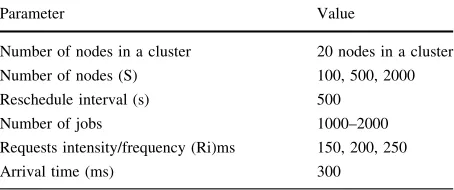
Windows 7 on an Intel i5 with 3 GB of RAM and 360 GB of hard disk has been used during simulation experiments in GridSim [30–34] version 5.0 [25] with JDK 1.5 updates 6 and JRE 1.3. The goal of this experiment is to compare the performance of a decen-tralized proposed load balancing algorithms (PLBA) with conventional Without Load Balancing (WLB) and Load balancing in enhanced GridSim (LBEGS) algorithm. All parameters are summarized in Table9.
Initially, all nodes having a zero load. Throughout the experiment, we use only one Grid user agent for the generation of Grid resource requests. For the simulated scenarios, it does not matter how many Grid user agents there are in the system. These experimental con-figurations are to bring up the performance of the load balancing algorithm as many as possible.
7.2 Simulation Results
The first experiment is to compare the performance of WLB, a LBGES algorithm with PLBA in terms of response time and resource allocation efficiency.
Figure4 depicts the response times that are influenced by Grid size, available con-nections and bandwidth using request intensity (Ri=200 ms). For comparing different Table 9 Simulation parameters
Parameter Value
Number of nodes in a cluster 20 nodes in a cluster
Number of nodes (S) 100, 500, 2000
Reschedule interval (s) 500
Number of jobs 1000–2000
Requests intensity/frequency (Ri)ms 150, 200, 250
Arrival time (ms) 300
0 2000 4000 6000 8000 10000 12000
100 500 1000 1500 2000
Response Time (ms)
Grid Size
Comparison of Response Time
WLB
LBGES
PLBA
size Grid, a lower average response time is considered to be better depicted through Fig.4. All algorithms present the best results in the small size Grid but, when the size of the Grid is larger, PLBA is decreasing quickly. The response time using PLBA can be 50 and 44 % shorter than that using the WLB and LBGES respectively.
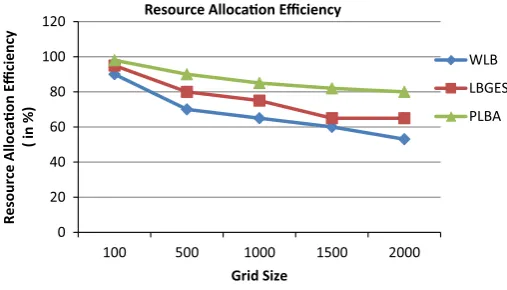
As shown in Fig.5, the PLBA outperforms the conventional WLB and LBEGS for the different size grid. Secondly, we measured the resource allocation efficiency of PLBA and WLB and LBEGS using Ri=200 ms. The WLB and LBEGS achieves to match nearly 98 % of all requests in the small size Grid scenario, with PLBA closely behind. However, as Grid size increases, the WLB and LBEGS degraded performance than the PLBA. Under the large size Grid, decrease of results for WLB and LBEGS is lower than in the small size. Resource allocation efficiency using PLBA is 27 and 15 % larger than that using the WLB and LBEGS. Varying Grid size, result decreases for both methods in similar manner.
The basic experiments described above have been conducted to show the fundamental differences between the PLBA and the WLB and LBEGS. Next, we devise sensitivity experiments in order to change the request frequency variables. The effects of request frequency to response time and resource allocation efficiency under different size of the Grid through below mentioned experiments. The following figure shows the behaviour of two allocation methods when changing the resource requests frequency from 50–100 to 200–400 ms.
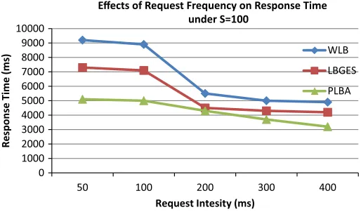
For the response time, a lower request frequency leads to faster access times whereas; X-axis shows a change in request frequency. Presented through Figs.6, 7 and 8, the response time using PLBA can be 21 and 9 % shorter than that using the WLB and LBEGS respectively, under small size Grid (S=100) and low request frequency (Ri=200 ms). When changing the size of Grid by S=500 and remain request frequency as Ri=200 ms, the response time of WLB and LBEGS is 19 and 11 % & longer than that using the PLBA. When increasing the size of Grid by S=2000 and request frequency by Ri=50 ms, the performance of WLB and LBEGS deteriorates quickly, the response time is 79 and 29 % longer than that using the PLBA. Under big size Grid (S=2000) and high request frequency (Ri=50, 100 ms), WLB and LBEGS take more time to allocate appropriate resources, the response time is 70 and 43 % longer than that using the PLBA. This effect could be caused by an increasing synchronization of the frequency request generation with the negotiations that lead to successful resource provisioning. In other
0
100 500 1000 1500 2000
Resource Allocaon Efficiency
0
Request Intensity (in ms)
Effects of Request Frequency on Response Time under S=500
WLB
LBGES
PLBA
Fig. 7 Frequency response time for constant Grid size=500 0
Effects of Request Frequency on Response Time under S=100
WLB
LBGES
PLBA
Fig. 6 Frequency response time for constant Grid size=100
0
Effects of Request Frequency on Response Time under S=2000
WLB
LBGES
PLBA
words, the large number of open requests leads to longer queues for processing, whereas the queues get shorter with decreasing request frequency, the overall processing gets faster. Considering the resource allocation efficiency, from the results in Figs.9,10and11, under small size Grid and low request frequency (Ri=200 ms), the resource allocation efficiency using PLBA is nearly the same as that using the WLB and LBEGS. When increasing the size of Grid by S=100 and remain request frequency as Ri=200 ms, the resource allocation efficiency of PLBA as much as 23 and 12 % larger that using the WLB and LBEGS respectively. When increasing the size of Grid by S=500 and request frequency by Ri=50 ms, the resource allocation efficiency of WLB and LBEGS is as much as 43 and 11 % less than that using the PLBA. Under big size Grid (S=2000) and high request frequency (Ri=50), the resource all location efficiency of WLB and LBEGS is as much as 43 % less than that using the PLBA. Resource allocation efficiency of 93 % can be achieved for the PLBA with a 200 ms pulse even in high request density. Complete saturation of
0
Resource Allocaon Efficiency %
Resource Intensity (in ms)
Effects of Request Frequency on Resource Allocaon Efficiency under S=100
WLB
LBGES
PLBA
Fig. 9 Resource allocation efficiency for constant Grid size=100
0
Resource Allocaon Efficiency %
Request Intensity (in ms)
Effects of Request Fequency on Resource Allocaon Efficiency under S=500
WLB
LBGES
PLBA
request in WLB and LBEGS can be attained in a small size Grid/high request density scenario. Increasing the request frequency implies a high charge to the system and in case of 50 ms pulses reduce the resource allocation efficiency to nearly 50 % in all scenarios. In most of the test cases, the PLBA is more efficient than the WLB and LBEGS to allocate Grid resources in the test application. When Grid size is creasing, it has more merits to use the PLBA to schedule Grid resource; the PLBA has better performance than usual WLB and LBEGS.
7.3 Comparison with Existing Algorithms
In Sect.7, we introduced an algorithm for resource selection including min–min, max– min, WLB, LBEGS, PLBA etc. In this section, the performance of WLB, min–min, max– min, LBEGS and PLBA in a Grid will be investigated by simulation. Suppose that there are ten resources that every resource has five machines, and every machine has four PEs, so leading to 200 PEs in total. The numbers of Gridlets are kept constant at 500 and every Gridlet at the beginning time and without a deadline request. Every PE is between grade 1 and 10 and every Gridlet is between grade 1 and 10 too. For ease of study, we set the local load factor of resources to be zero; this does not affect the performance of the algorithms. These settings are convenient for us to analyse the effectiveness and the behaviour of the algorithms. The resource load threshold parameters and Gridlet parameters are listed in Table8. The comparison of communication overhead times and makespan between above algorithms are depicted through Figs.12and13.
Figure12shows the communication overhead times of the different algorithms keeping the number of Gridlets up to 2000. It shows that the times of WLB and min–min increase quickly by increasing Gridlets; keeping max–min is in the middle. It can be observed that LBEGS and PLBA always have the minimum of the five algorithms and increase very slowly. Figure12shows that PLBA gives better performance by reducing communication overhead times and Fig.13shows the makespan of the different algorithms. It shows that the makespan of all algorithms increases with the number of Gridlets increasing; PLBA is the minimum of all algorithms that gives good performance with respect to makespan. In conclusion, PLBA has better performance in reducing communication overhead times and makespan.
Our experiments result is compared with Load Balancing in Enhanced GridSim (LBEGS). We have named our proposed solution as PLBA (Proposed Load Balancing Algorithm).
Resource Allocaon Efficiency %
Request Intensity (in ms)
Effects of Request Frequency on Resource Allocaon Efficiency under S=2000
WLB
LBGES
PLBA
7.4 Execution Time (LBEGS and PLBA) with Constant PEs
The results presented here are for the LBEGS and PLBA. Values for graph are taken by varying number of Gridlets starting at 250 and ending at 50 with a step of 50, and the numbers of PEs are kept constant at 20. The execution time is the average execution time of all the gridlets.
The graph of Fig.14shows that PLBA has a lower execution time. It is because (1) the Gridlets are assigned to a resource considering the current load, (2) imbalanced loads are mostly handled locally.
7.5 Execution Time (LBEGS and PLBA) with Constant Gridlets
The results presented here are for LBEGS and PLBA schemes. The readings are taken by varying number of PE starting at 10 and ending at 50 with a step of 10. The numbers of Gridlets are kept constant at 100. As it is displayed in Fig.15, it is evident that the gain in execution time is better in PLBA as compared to the LBEGS.
0
200 400 600 800 1000 1200 1400 1600 1800 2000
Communicaon Overhead
Times
No of GridLets
Communicaon overhead mes versus Gridlets on PEs = 200
Min-Max
Max-Min
LBGES
WLB
PBLA
Fig. 12 Communication overhead graph
0
200 400 600 800 1000 1200 1400 1600 1800 2000
Makespan
No of GridLets
Makespan versus Gridlets on PEs = 200
Min-Max
Max-Min
LBGES
WLB
PBLA
8 Conclusion and Future Work
In this paper multiple aspects of Grid Computing and numerous concepts which illustrate its broad capabilities has been described. Grid Computing is definitely a promising ten-dency to solve high demanding applications and all kinds of problems. Objective of the Grid environment is to achieve high performance computing by optimal usage of geo-graphically distributed and heterogeneous resources. But Grid application performance remains a challenge in dynamic Grid environment.
Resources can be submitted to Grid and can be withdrawn from Grid at any moment. This characteristic of Grid makes Load Balancing one of the critical features of Grid infrastructure. There are a number of factors, which can affect the Grid application performance like load balancing, heterogeneity of resources and resource sharing in the Grid environment.
In this paper the problem of load balancing in Grid computing has been addressed. Concepts of Grid Computing and their related paradigms have been studied. This report presented the impact of Load Balancing on Grid application performance and introduced
10 Execution Time Vs No. of gridlets
Number of PEs = 20
PLBA
LBGES Fig. 14 Execution time with
constant PEs
Execution time( in sec)
Number of PEs
Execution time vs. number of PE number of gridlets = 100
PLBA
LBGES Fig. 15 Execution time versus
the problematic of balancing the load among the participant in a Grid. A dynamic, dis-tributed load balancing approach for Grid has been proposed. The average execution time with constant number of Gridlets and with constant number of PEs has been improved in proposed approach which has shown in experimental results.
This paper proposes a threshold based dynamic load balancing algorithm for better response time, communication overhead and resource allocation efficiency etc., wherein resources, machines and the Grid broker participate in the load balancing operations. This approach minimizes the searching time to find out the receiver machine in order to transfer the Gridlets. A accurate examination of the proposed algorithm on the GridSim simulator has been carried out in order to judge the effectiveness of the algorithm. The simulation results have been provided to depict the effectiveness of the PLBA over WLB and LBEGS. PLBA enhances resource allocation capacity and better response time and communication overhead
Our proposed work can be extended to:
• Use adaptive policy (that uses both sender initiated and receiver initiated strategies). • Considered fault tolerance as a load balancing criterion.
• Add new scheduling approach.
References
1. Rathore, N., & Chana, I. (2015). Job migration policies for grid environment. Wireless Personal Communication,89(1), 241–269.
2. Rathore, N., & Chana, I. (2015). Variable threshold based hierarchical load balancing technique in grid. Engineering with Computers, 31(3), 597–615.
3. Rathore, N., & Chana, I. (2014). Load balancing and job migration techniques in grid: A survey of recent trends.Wireless Personal Communication, 79(3), 2089–2125.
4. Rathore, N., & Chana, I. (2014). Job migration with fault tolerance based QoS scheduling using hash table functionality in social grid computing.Journal of Intelligent & Fuzzy Systems, 27(6), 2821–2833. 5. Rathore, N. K., & Chana, I. (2013). Report on hierarchal load balancing technique in grid environment.
i-manager’s Journal on Information Technology, 2(4), 21–35.
6. Rathore, N. K., & Chana, I. (2010). Checkpointing Algorithm in Alchemi.NET. Pragyaan.Journal of Information Technology, 8(1), 32–38.
7. Rathore, N. K., & Chana, I. (2013). A sender initiate based hierarchical load balancing technique for grid using variable threshold value. InInternational conference IEEE-ISPC(pp. 1–6).
8. Rathore, N. K., & Chana, I. (2011). A cogitative analysis of load balancing technique with job migration in grid environment. In World congress on information and communication technology (WICT), Mumbai, IEEE proceedings paper(pp. 77–82).
9. Rathore, N. K., & Chana, I. (2008). Comparative analysis of checkpointing. InPIMR Third national IT conference, IT enabled practices and emerging management paradigm book and category is commu-nication technologies and security issues,Topic No/Name-46, Prestige Management and Research, Indore, (MP), India(pp. 32–35).
10. Rathore, N. K., & Chana, I. (2010). Fault tolerance algorithm in Alchemi.NET middleware. InNational conference on education & research (ConFR10), third CSI national conference of CSI Division V, Bhopal Chapter, IEEE Bombay, and MPCST Bhopal, organized by JUIT, India.
11. Rathore, N. K., & Chana, I. (2009). Checkpointing algorithm in Alchemi.NET. InAnnual conference of Vijnana Parishad of India and National Symposium Recent Development in Applied Mathematics & Information Technology, JUET, Guna, M.P.
12. Rathore, N. K., & Chana, I. (2008). Comparative analysis of checkpointing. InPIMR Third National IT conference, IT Enabled Practices and Emerging Management Paradigm book and category is Com-munication Technologies and Security Issues,Topic No/Name-46, Prestige Management and Research, Indore, (MP)India(pp. 32–35).
14. Rathore, N. K., & Chana, I. (2010). Checkpointing algorithm in Alchemi.NET. InLambert Academic Publication House (LBA), Germany.
15. Rathore, N. K. (2015). Efficient agent based priority scheduling and load balancing using fuzzy logic in grid computing.i-manager’s Journal on Computer Science, 3(3), 7–18.
16. Qureshi, K., Rehman, A., & Manuel, P. (2011). Enhanced gridsim architecture with load balancing.The Journal of Supercomputing, 57(3), 265–275.
17. Maoz, T., Barak, A., & Amar, L. (2008). Combining virtual machine migration with process migration for HPC on multi-clusters and grids. InIEEE international conference on cluster computing.Israel: The Hebrew University of Jerusalem.
18. Ali, H. H., El-Rewini, H., & Khalil, K. M. (1992). Controlled job migration in load balanced distributed systems. InIEEE.NE: University of Nebraska at Omaha.
19. Heiss, H.-U., & Schmitz, M. (1999).Decentralized dynamic load balancing: The particles approach. Department of Informatics, University of Karlsruhe, Germany.
20. Sairam, A. S., & Barua, G. (2010). Distributed route control schemes to load balance incoming traffic in multihomed stub networks. In:IEEE. Guwahati: Department of Computer Science and Engineering, Indian Institute of Technology Patna, Patna (Bihar), India.
21. Razzaqu, M. A., & Hong, C. S. (1991).Dynamic load balancing in distributed system: An efficient approach. Joint Conference on Communication and Information (JCCI), Phoenix Park, Korea. 22. Randles, M., Abu-Rahmeh, O., Johnson, P., & Taleb-Bendiab, A. (2010). Biased random walks on
resource network graphs for load balancing.The Journal of Supercomputing,53(1), 138–162. 23. Lee J., Keleher, P., & Sussman, A. (2010). Decentralized dynamic scheduling across heterogeneous
multi-core desktop grids. InParallel & distributed processing, workshops and Phd forum (IPDPSW), 2010 IEEE international symposium on.Atlanta, GA.
24. Ackermann, H., Fischer, S., Hoefer, M., & Scho¨ngens, M. (2011). Distributed algorithms for QoS load balancing.Distributed Computing,23(5–6), 321–330.
25. Saruladha, K., & Santhi, G. (2007). Behavior of agent based dynamic load balancing algorithm for heterogeneous P2P. InInternational conference on computational intelligence and multimedia appli-cations. Pondicherry: CSE Dept., Pondicherry Engineering College.
26. Petrova, M., Olano, N., & Mahonen, P. (2010). Balls and bins distributed load balancing algorithm for channel allocation. InIEEE. RWTH Aachen University Aachen.
27. Shah, R., Veeravalli, B., & Misra, M. (2007). On the design of adaptive and decentralized load-balancing algorithms with load estimation for computational grid environments.IEEE Transactions on Parallel and Distributed Systems, 18(12), 586–598.
28. Yagoubi, B., & Slimani, Y. (2007). Load balancing strategy in Grid environment.Journal of Infor-mation Technology and Applications, 1(4), 285–296.
29. Jain, P., & Gupta, D. (2009).An algorithm for dynamic load balancing in distributed systems with multiple supporting nodes by exploiting the interrupt service. New Delhi: ACEEE, Academy Publisher, Delhi College of Engineering.
30. Rathore, N. K. (2016). Ethical hacking & security against cyber crime.Journal on Information Tech-nology,5(1), 7–11.
31. Rathore, N. K. (2015). Map reduce architecture for grid.Journal on Software Engineering,10(1), 21–30.
32. Rathore, N. K. (2015). GridSim installation and implementation process.Journal on Cloud Computing, 2(4), 29–40.
33. Sharma, V., Kumar, R., & Rathore, N. K. (2015). Topological broadcasting using parameter sensitivity based logical proximity graphs in coordinated ground-flying ad hoc networks. Journal of Wireless Mobile Networks Ubiquitous Computing and Dependable Applications (JoWUA), SCOPUS Indexed, 6(3), 54–72.