Load balancing strategies for SPH

Load Balancing Strategies for SPH

Kunal Puri

Department of Aerospace Engineering Indian Institute of Technology Bombay

Powai, Mumbai 400076 Email: kunal.r.puri@gmail.com

Prabhu Ramachandran

Department of Aerospace Engineering Indian Institute of Technology Bombay

Powai, Mumbai 400076

Email: prabhu.ramachandran@gmail.com

Pushkar Godbole

Department of Aerospace Engineering Indian Institute of Technology Bombay

Powai, Mumbai 400076 Email: pushkar.godbole91@gmail.com

Abstract—We evaluate the performance of different load balancing algorithms when used with the Smooth Particle Hydro-dynamics (SPH) particle method. We compare several geometric algorithms and a serial graph partitioning algorithm (Metis) in terms of the efficiency and quality of partitioning. We find that the geometric partitioners are better suited with the RIB method producing the best partitions for the problems considered.

I. INTRODUCTION

Lagrangian, mesh-free method for the numerical solution of partial differential equations. The Lagrangian nature of SPH renders it suitable for large deformation problems in arbitrary domains. The domain is discretized with “particles” that carry with them physical properties. The evolution of these properties through particle-particle interactions, in accordance with the governing differential equations describes the system. One of the principal applications of SPH is for free surface flows [1], [2], [3], in which an incompressible fluid moves under the influence of gravity in an open vessel. An accurate description of the flow requires a large number of particles (a typical 3D dam break problem can have half a million particles) and one must look for parallel paradigms for any realistic SPH implementation. In a parallel implementation, each processor is assigned a set of particles (local particles) to evolve. Moreover, to carry out pair-wise interactions across processor boundaries, “ghost” particle data (remote particles) must be shared as a buffer or halo region around a neighboring processor. The assignment of particles to processors must ensure a balanced workload and a minimal surface area to reduce the time spent communicating ghost/buffer particles. Furthermore, the load balancing algorithm should be dynamic to exploit the Lagrangian nature of the simulation.

In this work, we evaluate the feasibility of different geometric and graph partitioning algorithms for their use with SPH. We use the Zoltan data management library [7], [8] which implements geometric and graph based partitioning algorithms. The algorithms are assessed based on the time taken for the decomposition, the distribution of work-load across processors and the communication overhead required for exchanging ghost neighbors. Although the discussion on load balancing is agnostic to a particular application area, we choose the dam break problem as a concrete test case. The dam break problem adds a sufficient amount of complexity like multiple species (fluid, solid) and boundary conditions without obfuscating the SPH algorithm itself. To the best of our knowledge, a comparative evaluation of load balancing algorithms for SPH does not exist.

The outline of the paper is as follows. In Sec. II, we outline the parallel SPH algorithm for distributed memory machines we

adopt for this work. In Sec. III, we discuss the load balancing algorithms used in this work.

II. SMOOTHPARTICLEHYDRODYNAMICS

We briefly outline a typical SPH operation and the parallel algorithm adopted in this work. The parallel implementation assumes a distributed memory machine equipped with the message passing libraries (MPI).

A. Basic SPH

SPH is based on the theory of kernel interpolation whereby a sufficiently smooth function f can be approximated at an arbitrary point x in a domain Ω by summing contributions

from near-neighbors

f(x)≈

X

b∈N(x)

fbW(|x−xb|, h)∆b (1)

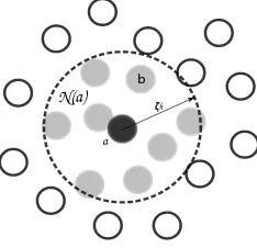
The interpretation is that the function values are weighted by a kernel function W, and ∆b is the nodal volume associated with an interpolation point. The kernel is compactly supported which implies a summation over nodes only in the neighbor-hood of the evaluation pointx(denoted asN(x)) as shown in

Fig. 1 Gradients can be constructed in similar vein to result in

a b N(a)

ζh

Fig. 1. The set of neighbors (Na) for a given particle is determined by it’s interaction radius.

evolution equations in the form of short-range forces between particle pairs. We refer the interested reader to [4], [5]. An example of (1) is to approximate the density at a point as

ρa= X

b∈N(a)

mbW(xa,xb, ha) (2)

density (ρ) and the nodal volumes are approximated as the ratio of particle mass to density (∆b=mb/ρb).

For the dam-break problem, we solve the incompressible Navier-Stokes equations

using the weakly compressible approach [6], [2]. The pressure is coupled to the density using the Tait equation of state

P =B

The equations are integrated using a second order predictor corrector or Runge-Kutta integrator.

B. Parallel SPH

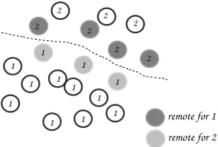
In our parallel SPH implementation, every processor is responsible for the evolution of a subset of the total number of particles. Particles assigned to a processor are called local particles. To carry out the short-range force computations across processor boundaries, particles must be shared as buffer or halo regions as shown in Fig. 2. These particles are called remote particles. We assume all particles to require the same

1

Fig. 2. Local and remote particles for an imaginary particle distribution. Particles assigned to a processor are localwhile those shared for neighbor requirements areremote

processing time per time step. This is valid for the weakly compressible formulation. With this assumption, the number of local particles on a processor determines the load balance while the exchange of remote particles provides a measure of the quality of a partition. Owing to the Lagrangian nature of SPH, the particles move over the computational domain and the remote particles must be re-computed at every time step to satisfy the neighbor requirements. Dynamic load balancing is needed to achieve a good partition to keep the communication overhead low. Once the ghost particles have been exchanged for a given decomposition, the serial algorithm can be applied on each processor to update the local particles.

The steps for the parallel SPH implementation is listed in Algo-rithm. 1. We assume some given decomposition as initial input. If the partition is not balanced (based on estimates available), we call the load balancer to re-distribute the particles. Remote particles are then exchanged. Once the new decomposition is

available, we perform the serial SPH calculations to determine the forces on the local particles. When the particle positions

Algorithm: Parallel Update

ifnot balanced then

call LoadBlance

call ComputeRemoteParticles

end

call SerialSPH

call UpdateLocalParticles

foreach local particledo

call FindNewPartition call UpdatePartition

end

Algorithm 1: Update sequence in our parallel SPH imple-mentation

are updated, we determine the partition to which they must be assigned and update it. Counting the number of particles to be re-assigned gives us a measure to check if load balancing is required in a subsequent time step. The update algorithm is straightforward and hinges on efficient dynamic load balancing algorithms which are discussed next.

III. LOADBALANCINGALGORITHMS FORSPH

Load balancing algorithms strive to achieve a balanced workload among available processors while minimizing the communication overhead for the additional data required for the calculation. For SPH, the number of local particles assigned to a processor determines the work and the exchange of remote particles determines the communication overhead. Depending on the input, load balancing methods are classified as geo-metric or graph based. Common to both is that the objective is to obtain an assignment of certain “objects” to available processors which, in the case of SPH, are particles.

A. Geometric Partitioners

Geometric partitioners take as input, the coordinate po-sitions of the objects to be partitioned. The algorithms are physically intuitive and are the natural choice for particle methods like SPH.

1) Recursive Coordinate Bisection (RCB): The RCB al-gorithm is the simplest of the geometric partitioners. It begins bisecting the domain using a plane orthogonal to the coordinate axes. This generates two sub-regions with equal number of particles. This algorithm is then applied recursively to each sub-region to reach the desired number of partitions. Weights can be assigned to particles to achieve different load balancing criteria. For our purpose, we do not assign weights for the RCB method. The principle advantage of the RCB method is speed and simplicity. A disadvantage of the RCB method is that it can generate disconnected sub-domains.

3) Hilbert Space Filling Curve (HSFC): Space filling curves are functions that map a given point in a domain into the unit interval [0,1]. The inverse functions map the unit interval to the spatial coordinates. The HSFC algorithm divides the unit interval into P intervals each containing objects associated to these intervals by their inverse coordinates [8]. N bins are created to partition the interval and the weights in each bin are summed across all processors. The algorithm then sums the bins and places a cut when the desired weight for a partition is achieved. The process can be repeated to improve the partitioning tolerance.

B. Graph Partitioners

Graph partitioning techniques used for mesh based schemes re-interpret the mesh data structure as a graph, with the elements defining the nodes and the element connectivity as the edges between the nodes. The algorithm then proceeds to partition the graph by performing cuts along the edges. Since the connectivity information is implicit in the definition of a graph, the application of these algorithms to meshless methods is not clear. In SPH, the particles could be treated as the vertices in the graph while the nearest neighbors could define the edges emanating from a given vertex. While this works in principle, the resulting graph can have too many edges, leading to expensive running times for the algorithm. An alternative is to use the particle indexing structure as an implicit mesh where the cells define the nodes and the cell neighbors (27in3D and9in2D) define the node connectivity. The graph is now invariant to the number of neighbors for a given particle (resolution in SPH). Edges can be weighted based on the number of particles in each cell to achieve a good load balance across processors. The cells however, must be unique across the computational domain which raises the communication overhead. Additional overhead is incurred for these methods in determining the remote particles required to complete the load balancing phase. The main advantage of graph partitioners is that they produce fast and high quality partitions.

For our experiments, we use the serial graph partitioner Metis [9] to obtain a distribution of particles which are then scattered to their respective processors. Although Zoltan implements a parallel graph and hyper-graph partitioner, their inclusion was beyond the scope of this work.

IV. EXAMPLES ANDRESULTS

In this section we compare the particle distributions pro-duced by the different load balancing algorithms for two test cases. While the results presented are for two dimensions, the implementation is readily applicable in 3D. The 2D examples facilitate an understanding of the distributions produced by the different algorithms.

A. The box test

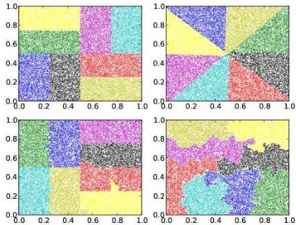
The first example is a box-test in which particles are randomly distributed in the unit interval. The initial particle to processor assignment is random. This generates a highly imbalanced distribution with which we check the performance of the different load balancing algorithms. Fig. 3 shows repre-sentative partitions generated using the RCB, RIB, HSFC and Metis partitioners for 216 _{particles on4 processors. Although}

Fig. 3. Particle distribution for216

particles on4_{processors. Particles are}

colored according to processor assignment.

this is a very simple domain, the differences between the algo-rithms is evident. The RCB method produces sub-domains that are axis-aligned. The RIB method has performed cuts along the diagonal of the domain which results in the triangular sub-domains. The HSFC method produces a partition very similar to RCB but with a slight overlap of processor domains. Metis has produced a very irregular distribution with disconnected regions. We note that we used particle coordinates as the graph vertices and particle neighbors as the graph edges for the input to Metis. An alternative would be to use the cell indexing structure as an input mesh for Metis. Fig. 4 shows the partitions generated on8processors for the same problem. The

Fig. 4. Particle distribution for216

particles on8_{processors. Particles are}

colored according to processor assignment.

qualitative features of the partitions are the same. In particular, we find that the Metis output is poor with disconnected sub-domains.

advantage is that the graph is now invariant to the number of neighbors for a given particle and the resulting decomposition is better as can be seen in Fig. 5. The partitioning quality as a

Fig. 5. Graph partitioning using cell neighbors (left) versus cell neighbors (right) using Metis. Notice that using the cell indexing structure produces a better distribution without disconnected sub-domains.

function of cell size for 106 _{particles is shown in Fig. 6 The}

0 10 20 30 40 50 60

cell size in terms of IR 500

0 500 1000 1500 2000 2500 3000 3500

Deviation (particle distribution)

Fig. 6. Partition quality for Metis using cell partitioning for106 particles. The quality is determined as the deviation from the mean of the number of particles for each processor.

quality is determined as the load balance across processors. From the figure we can see that the deviation (excess particles) increases quadratically with the cell size. As we increase the cell size in the input to Metis, the time taken for the partitioning reduces as seen in Fig. 7 This suggests a trade-off between increasing the cell size for faster partitioning times vis-a-vis load balance across processors.

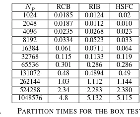
The partitioning times for the geometric algorithms (RCB, RIB and HSFC) are shown in Table. I. The table shows that the RCB is the fastest method for this problem although the actual times are comparable.

0 1000000 2000000_particles3000000 4000000 5000000 0

5 10 15 20 25 30 35 40 45

seconds

Partitioning performance Cell partitioning R = 2 x IR Cell partitioning R = 5 x IR Cell partitioning R = 10 x IR Cell partitioning R = 15 x IR Cell partitioning R = 20 x IR

Fig. 7. Partitioning times for Metis using cells as the number of particles is increased. Increasing the cell size results in faster partitioning times.

Np RCB RIB HSFC

1024 0.0185 0.0124 0.02 2048 0.0187 0.0112 0.010 4096 0.0235 0.0268 0.023 8192 0.0334 0.0523 0.033 16384 0.061 0.0711 0.064 32768 0.115 0.1133 0.119 65536 0.301 0.286 0.286 131072 0.48 0.4894 0.49 262144 1.03 1.112 1.144 524288 2.34 2.283 2.380 1048576 4.8 5.132 5.115

TABLE I. PARTITION TIMES FOR THE BOX TEST USING THE

GEOMETRIC PARTITIONERS.

B. Dam break problem

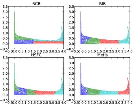
The dam-break problems are an important area of applica-tion area of SPH. In these problems, an incompressible fluid moves under the influence of gravity in an open vessel. The fluid may encounter obstacles in it’s path as for example, a wave striking a lighthouse tower. The challenge is to capture the large deformations of the fluid free surface as a result of interactions with solid objects. The schematic of the problem we consider is shown in Fig. 8 Dynamic load balancing is needed in this problem because the particles move over the computational domain. Fig. 9 shows the particle distribution using 4 processors when the fluid column has hit the vessel wall. The qualitative features from the box test are reproduced for this example with the exception that Metis shows a marked improvement for this problem producing a decomposition very similar to the RIB method. Fig. 10 displays the decomposition for this problem using8 processors. From the distribution we see that the RCB method once again produces a domain de-composition that is axis-aligned but in this case results in sub-domains that are disconnected. RIB and Metis produce nearly identical partitions. The HSFC method results in disconnected regions for this case.

V. CONCLUSION

2

4 1 m

m

m

Fig. 8. Schematic for the dam break problem.

Fig. 9. Particle distribution for the dam break problem with4_processors.

processors is the required objective. The algorithms tested were the Recursive Coordinate Bisection (RCB), Recursive Internal Bisection (RIB), Hilbert Space Filling Curve (HSFC) and the static graph partitioning algorithm of Metis.

For the box test (Sec. IV-A), graph partitioning using Metis produced disconnected sub-domains when using the particle neighbors to define the edges of the graph. We found that using the cell indexing structure is an effective way to use graph partitioning for SPH. The cell size must be chosen appropriately to achieve a good load balance and reasonable running times for the algorithm.

Geometric partitioners are a natural choice for particle methods as the input to these algorithms are the particle coordinates. For the dam break problem, the RIB method produced de-compositions comparable to those generated by Metis while the RCB and HSFC methods resulted in disconnected regions when the number of partitions were increased.

Fig. 10. Particle distribution for the dam break problem with8_processors.

REFERENCES

[1] Angela Ferarri and Michael Dumbser and Eleuterio F. Toro and Aronne Armanini. A new 3D parallel SPH scheme for free surface flows. Computers and Fluids, 38:1023–1217, 2009.

[2] J.J. Monaghan. Smoothed Particle Hydrodynamics and Its Diverse Applications. Annual Review of Fluid Mechanics, 44:323–346, 2012. [3] Moncho Gomez-Gesteria and Benidict D. Rogers and Robert A.

Dalrym-ple and Alex J. Crespo State-of-the-art of classical SPH for free surface flows.Journal of Hydraulic Research, 48:6–27, 2010

[4] J.J. Monaghan. Why Particle Methods Work SIAM Journal of Scientific and Statistical Computing, 3 1982

[5] J.J. Monaghan. Smoothed Particle HydrodynamicsReports on Progress in Physics, 68, 1703–1759, 2005

[6] J.J. Monaghan. Simulating free surface flows with SPH Journal of Computational Physics, 110:399–406

[7] Karen Devine and Erik Boman and Robert Heaphy and Bruce Hen-drickson and Courtenay Vaughan Zoltan Data Management Services for Parallel Dynamic Applications Computing in Science and Engineering, 4, 90–97, 2002

[8] Erik Boman, Karen Devine, Lee Ann Fisk, Robert Heaphy, Bruce Hendrickson, Vitus Leung, Courtenay Vaughan, Umit Catalyurek, Doruk Bozdag, and William Mitchell. Zoltan home page.

http://www.cs.sandia.gov/Zoltan, 1999.