Model Components Selection in
Bayesian Model Averaging Using
Occam's Window for Microarray Data
Ani Budi Astuti1, Nur Iriawan2, Irhamah3, Heri Kuswanto4
1
Department of Mathematics, Faculty of Mathematics and
Natural Sciences, University of Brawijaya,
Malang, Indonesia
1
PhD. Student at Department of Statistics, Faculty of Mathematics
and Natural Sciences, Institut Teknologi Sepuluh Nopember, Surabaya, Indonesia
2,3,4
Department of Statistics, Faculty of Mathematics and
Natural Sciences, Institut Teknologi Sepuluh Nopember, Surabaya, Indonesia 1
e-mail: [email protected]
Abstract— Microarray is an analysis for monitoring gene expression activity simultaneously. Microarray data are generated from microarray experiments having characteristics of very few number of samples where the shape of distribution is very complex and the number of measured variables is very large. Due to this specific characteristics, it requires special method to overcome this. Bayesian Model Averaging (BMA) is a Bayesian solution method that is capable to handle microarray data with a best single model constructed by combining all possible models in which the posterior distribution of all the best models will be averaged. There are several method that can be used to select the model components in Bayesian Model Averaging (BMA). One of the method that can be used is the Occam's Window method. The purpose of this study is to measure the performance of Occam's Window method in the selection of the best model components in the Bayesian Model Averaging (BMA). The data used in this study are some of the gene expression data as a result of microarray experiments used in the study of Sebastiani, Xie and Ramoni in 2006. The results showed that the Occam's Window method can reduce a number of models that may be formed as much as 65.7% so that the formation of a single model with Bayesian Model Averaging method (BMA) only involves the model of 34.3%.
Keywords— Bayesian Model Averaging, Microarray Data, Model Components Selection, Occam's Window Method.
1
I
NTRODUCTIONMicroarray data is the data obtained from a microarray experiment that is an experiment with a particular analysis technique to monitor the activity of thousands genes expression simultaneously [1]. Microarray data have several characteristics i.e. -limited availability of the number of samples because of limited budget, resources and time. Though the availability of the number of samples is limited, the measurable characteristic variables can be hundreds or even thousands of gene expression. By these special characteristics, it is possible that the nature of the distribution of gene expression data will be very complex in which the distribution of the data is probably not a normal distribution [2]. Due to these specific characteristics, it requires special method to overcome this.
Bayesian is a statistical analysis method that does not consider the number of samples (especially for very small sample size) and to any form of distribution. Moreover, Bayesian method is based on information from the original data (driven data) to obtain the posterior probability distribution which is a product of the prior distribution and the likelihood function [3]. Model Parameter in Bayesian method is viewed as a random variable in the space of model parameter and allows for the formal combination of different from the prior distribution and facilitates the iterative updating of new information which thus overcome the problem of uncertainty and complexity of the model in the data [4] .
method is quite simple and widely used in research related the BMA in which obtained quite good results in the model components selection in the modeling of the BMA [5] and [6].Various studies have been done related to the Bayesian Model Averaging (BMA), among others [6], [7], [8], [9], [10] and [11]. In this study will be used Occam's Window method of [5] to select the component model in the modeling of the BMA for microarray data.
2
M
ICROARRAY,
B
AYESIANM
ODELA
VERAGINGA
NDO
CCAM’
SW
INDOWM
ETHOD2.1 Microarray Techniques and Microarray Data
According to [1], microarray technique is a technique of data collection by using the platform (reference) which is a duplicate of the original object identifier. The measurement data of a microarray technique called Microarray Data [12]. There are a variety of different technologies have been developed for microarray techniques, among which is a Synthetic Oligonucleotide Microarray Technology [13]. Gene expression data is the measurement data from Microarray techniques so that the gene expression data has the characteristics of microarray data. According to [2], the data obtained from experiments with microarray technique has the following characteristics:
1. The number of samples that can be observed very limited (slightly) because of limited budget, resources and time. Though the availability of the number of samples is limited, the measurable characteristic variables can be hundreds or even thousands of gene expression.
2. The nature of the distribution of data will be very complex in which the distribution of the data is probably not a normal distribution.
By looking at the characteristics possessed by the microarray data then to analyze of the microarray data requires special handling because it is generally the basis of parametric statistical method, especially for the comparative analysis requires a large number of samples. If the basis of this statistical method is not fulfilled then the conclusion of the analysis cannot be accounted for [9].
2.2 Bayesian Method
Bayesian is a statistical method based on the combination of two information that are the past of data information as the prior information and the observations data as a constituent likelihood function to update the prior information in the form of posterior probability distribution model. Bayesian method is based on information from the original data (driven data) to obtain the posterior probability distribution and it is does not consider the number of samples (especially for very small sample size) and to any form of distribution. Bayesian method allows for the formal combination of different from the prior distribution and facilitates the iterative updating of new information, which thus overcome the problem of uncertainty and complexity of the model in the data. The Rational of Bayesian method derived from Bayes Theorem thinking concept invented by Thomas Bayes in 1702-1761[3], [4], [14] and [15].
In Bayesian method, the parameters of the model
θ
are seen as a random variable in the parameter spaceθ
. Suppose there are x observational data with likelihood functionf(x|θ
)then the known information about the parameters before the observations were made is referred to as priorθ
namely p(θ
). Posterior probability distribution ofθ
, namelyp(θ
|x)determined by the rules of probability in Bayestheorem [3] as in equation (2.1).
θ
p
(
θ
|
x
)
=
f
(
x
|
θ
)
p
(
θ
)
where
f(x) is a constant called the normalized constant [4]. So that the equation (2.1) can be written as:
p(θ|x)∝ f(x|
θ
)p(θ) (2.2)Equation (2.2) shows that the posterior probability is proportional to the product of the likelihood function and the prior probability of the model parameters. This means that the update's information prior to use information of samples in the data likelihood to obtain the posterior information that will be used for decision making [16].
2.2.1 Markov Chain Monte Carlo (MCMC) Algorithms with Gibbs Sampler Approach
According to [17], [18] and [19], MCMC algorithms with Gibbs sampler approach can be described as:
Step 1. Set initial values for
θ
(k)at k=0 so that
θ
(0 )=
θ
1(0 ),...,θ
r(0 )(
)
Step 2. Sampling process to obtain the value of
θ
j from the conditional distribution by the samplingfor
θ
(k+1)2.3 Bayesian Model Averaging (BMA)
2.3.1 Basic Concepts of Bayesian Model Averaging (BMA)
The basic concept of Bayesian Model Averaging (BMA) is the best single model formed by considering all possible models that could be formed. BMA is a Bayesian solution for model uncertainty in which the completion of the model uncertainty by averaging the posterior distribution of all the best models. The purpose of the BMA is to combine models of uncertainty in order to obtain the best model [5] and [6].
According to [20], the prediction parameters using the BMA approach uses data derived from a combination of hierarchical models. If known {M1,M2,...,Mq}is the set of models which, may be formed
fromM and is the value to be predicted, then the BMA prediction begins with determining the prior probability distribution of all the parameters of the model and the model M
k. Posterior distribution of Δ if
the average of the posterior distribution if known models weighted by posterior probability models. While the posterior probability of the model Mk is:
P(x|Mk)=∫P(x|
θ
k,Mk)P(θk|Mk)dθ
k (2.5)Equation (2.5) is the marginal likelihood of the model M
k. Prior probability of
θ
k if known model Mk is p(θ
k|Mk) and p(θ
k|Mk) is the likelihood and p(Mk)is the prior probability ofMkif model Mkis true.
Implicitly, all probabilities depend on the model M so that the expected value of the coefficient of Δ
obtained by averaging the model of M , that is:
E(Δ|x)= P(Mk|x)E(Δ|Mk,x) k=1
q
∑
(2.6)The value of E(Δ|x) in the equation (2.6) shows the weighted expected value of Δ in every model possible
combination (weights determined by the prior and the model). While the variance of (Δ|x) is:
Var(Δ|x)= (var(Δ|x,Mk)+[E(Δ|Mk,x]
2
)P(Mk|x)−E(Δ|x)
2
)
k=1
q
∑
(2.7)2.3.2 Model Components Selection in Bayesian Model Averaging (BMA).
Based on the basic concept of Bayesian Model Averaging (BMA), the components of the model will be selected to be included in the equation (2.3) of q number of models that may be formed. There are several method for selecting the components model that will be includeed in the equation (2.3) based on its posterior probabilities, which are Occam's Window method [5]. Occam's Window method is quite simple and widely used in research related to the BMA and give good results in the selection of components model in the BMA [5] and [6]. According to [5], the rationale of Occam's Window method in selecting the component model in the BMA modeling based on the posterior probability of the model. The model that will be accepted by this method (the model can fit in modeling BMA) must satisfy the following equation:
A’= {M k:
maxl(P(Ml|x)) P(Mk|x) ≤
c} (2.8)
where A’ is the posterior odds to the model-k and c values of 20 is equivalent to
α
=5% if using the test criteria with p-value [21]. If a model has a value of A’ is greater than 20, then the model is not included in the modeling of the BMA and must be removed from the equation (2.3) and otherwise if a model has a value of A’ is less than or equal to 20, then the model will be included in the modeling of the BMA and should be included in the calculation of equation (2.3). In the equation (2.8), maxl(P(Ml|x)) is the model with thehighest posterior probability score andP(Mk|x) is the value of the posterior probability of the model-k. In
the various applications of Occam's Window method is generally able to reduce the large number of components model so that it becomes less than 100 models of even less than 10 models. Reduction of component model that only one or two models are very rare but may occur [5].
3
P
ROCEDUREThe data used in this study are some of the data used in the study [22]. Selection of component models in the BMA modeling begins with determining the most appropriate form of distribution to the data and parameter estimator and then based on the distribution model raised several distribution models by MCMC method with the Gibbs sampler approach to obtain some models that might be formed. Selection of component in the BMA modeling using Occam's window method [5] with the following formula:
A’={M k:
maxl(P(Ml|x)) P(Mk|x) ≤
c}. The BMA Modeling in the equation (2.3) is based on the result of model
4
R
ESULTSA
NDD
ISCUSSION4.1 Description of Gene Expression Data on Diseased and Health Conditions with Poly Detector
and mRNA Method
Results of Descriptive statistics for gene expression data on the deseased and healthy condition can be seen in the following figure:
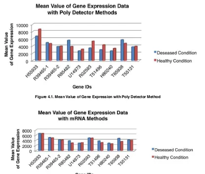
Figure 4.1. Mean Value of Gene Expression with Poly Detector Method
Figure 4.2. Mean Value of Gene Expression with mRNA Method
Based on Figure 4.1 and Figure 4.2 for the 10 ID genes were observed known that there are differences in gene expression for diseased and healthy conditions in which there are several ID genes showed that in healthy condition is more expressive than the diseased condition that is H55933, R39465-2, U14973, R02593, T51496, H80240 and T55131 for Poly Detector method and U14973 for mRNA method and otherwise there are several ID genes showed that in diseased condition is more expressive than the healthy condition that is R39465-1, R85482 and T65938 for Poly Detector method and H55933, R39465-1, R39465-2, R85482, R02593, T51496, H80240, T65938 and T55131 for the mRNA method.
4.2 Identification of Distribution and Parameter Estimator for the Data
Based on Table 4.1 and Table 4.2, it can be seen that there are some differences in the distribution of ID genes in diseased and healthy conditions that is 6 ID genes with Poly Detector method and 5 on the mRNA method and some other ID genes that have the same distribution that is 4 ID genes in Poly Detector method and 5 on the mRNA method. In addition, most of the data have a non-normal distribution that is lognormal distribution and there are some others have 2-parameter exponential distribution.
TABLE 4.1.DISTRIBUTION SHAPE AND ESTIMATOR PARAMETER FOR GENE EXPRESSION DATA WITH POLY DETECTOR METHOD
No Gene IDs
Diseased Condition Poly Detector Methods
Healthy Condition Poly Detector Methods Distribution
Shape Location Scale Threshold
Distribution
Shape Location Scale Threshold
1. H55933 Lognormal 8.68823 0.53647 - Lognormal 8.98607 0.42519 - 2. R39465-1 Lognormal 8.42867 0.43524 - Normal 4687.485 1140.79842 - 3. R39465-2 Normal 3853.22364 1332.10555 - Lognormal 8.25584 0.26893 - 4. R85482 Lognormal 8.54118 0.42501 - Normal 3896.826 1470.0419 -
5. U14973 2-parameter
Exponential - 1652.94571 1016.28221 Lognormal 7.95942 0.46248 - 6. R02593 2-parameter
Exponential - 2095.14952 1366.67186 Normal 5334.62 2808.25975 - 7. T51496 2-parameter
Exponential 7.78386 0.62935 - Normal 4319.807 1849.69333 - 8. H80240 Normal 2657.95909 763.91763 - Normal 3358.974 1453.48354 - 9. T65938 Lognormal 8.51113 0.56238 - Lognormal 8.3776 0.43201 - 10. T55131 Normal 3757.73 1316.13062 - Normal 3937.965 1043.66701 -
TABLE 4.2.DISTRIBUTION SHAPE DAN ESTIMATOR PARAMETER FOR GENE EXPRESSION DATA WITH MRNAMETHOD
No Genes ID
Diseased Condition mRNA Methods
Healthy Condition mRNA Methods Distribution
Shape Location Scale Threshold
Distribution
Shape Location Scale Threshold
4.3 Model Components Selection in BMA with Occam's Window Method
The results of the identification to model components selection in BMA with Occam’s Window method can be seen in Table 4.3 and Table 4.4.
Poly Detector Methods Poly Detector Methods Healthy Condition
The number Overall Mean 32.54 Overall Mean 63.64
component models in the BMA modeling was 65.7% so that in the formation of the BMA modeling involves only 34.3% of the overall model might be formed.
5
CONCLUSION
Based on the results of research conducted, it can be concluded that most of the gene expression data as a result of microarray experiments have non-normal distributions both in healthy and diseased conditions. In addition, there are different type of data distribution in healthy and diseased conditions and there is also the same type of data distribution in healthy and diseased conditions. There are several gene IDs that have the value of the expression in diseased condition stronger than healthy condition and otherwise there are several gene IDs that have the value of the expression in healthy condition stronger than diseased condition. The average percentage of the component model that can be included in the BMA modeling with Occam's Window method as much as 34.3%. This means that the Occam 's Window method can reduce the component model may be formed as much as 65.7% so that in the form of the BMA modeling involve only 34.3% where it would further simplify the model without reducing the validity of the model is formed.
6
ACKNOWLEDGMENT
This paper is part of the doctoral research at the Department of Statistics, Institut Teknologi Sepuluh Nopember (ITS) Surabaya, Indonesia. We would like to thank to group research Sebastiani P., Xie H. and Ramoni M.F. to use his data and to anonymous reviewers of this paper.
7
REFERENCES
[1] Knudsen, S., “A Guide to Analysis of DNA Microarray Data”, Second Edition, John Wiley & Sons, Inc., New Jersey, Canada, 2004. [2] Muller, P., Parmigiani, G., Robert, C., and Rouseau, J., “Optimal Sample Size for Multiple Testing: the Case of Gene Expression
Microarrays,” Tech. rep., University of Texas, M.D. Anderson Cancer Center, 2002.
[3] Gosh, J. K., Delampady, M. and Samanta, T., “An Introduction to Bayesian Analysis Theory and Method”. Springer, New York, 2006. [4] Gelman, A., Carlin, J. B., Stern, H. S. and Rubin, D. B., “Bayesian Data Analysis”, Chapman & Hall, London, 1995.
[5] Madigan, D. and Raftery, A. E., “Model Selection and Accounting for Model Uncertainty in Graphical Models Using Occam’s Window”, Journal of the American Statistical Association, Vol.89. 428: 1535-1546, 1994.
[6] Hustianda, V. F., “Comparison of Bayesian Model Averaging and Multiple Linear Regression in Predicting Factors Affecting Number of Infant Death in East Java”, Thesis, Statistics Department, FMIPA-ITS, Surabaya, 2012.
[7] Liang, F. M, Troung, Y, and Wong, W. H., “Automatic Bayesian Model Averaging for Linear Regression and Applications in Bayesian Curve Fitting”, Statistical Science, 11(4): 1005-1029, 2001.
[8] Brown, P.J., Vannucci, M. and Fearn, T., “Bayesian Model Averaging with Selection of Regressors”, J. R. Statist. Soc. B Part 3. 519–536, 2002.
[9] Sebastiani, P., Xie H. and Ramoni, M.F., “Bayesian Analysis of Comparative Microarray Experiments By Model Averaging”, International Society For Bayesian Analysis 1, number 4, pp. 707-732, 2006.
[10] Purnamasari, R., “The use of Bayesian Model Averaging (BMA) method with Markov Chain Monte Carlo (MCMC) approach for Wind Speed Daily Averages Forecasting in Juanda Meteorological Station”, Thesis, Statistics Department, FMIPA-ITS, Surabaya, 2011. [11] Kuswanto, H. and Sari, M. R., “Bayesian Model Averaging with Markov Chain Monte Carlo for Calibrating Temperature Forecast from
Combination of Time Series Models”, (on Review), 2013.
[12] Shoemaker, J. S. and Lin, S. M., “Method of Microarray Analysis IV”, Springer, New York, 2005.
[13] Duggan, J. D., Bittner, M., Chen, Y., Meltzer, P. and Trent, J. M., “Expression Profiling Using CDNA Microarrays. Nature Genetics”, 21: 10-14, 1999.
[14] Box, G. E. P. and Tiao, “Bayesian Inference in Statistical Analysis”, MA: Addison-Wesley, Massachusetts, 1973. [15] Zellner, A., “An Introduction to Bayesian Inference in Econometrics”, John Wiley, New York. 1971.