DOI 10.1007/s11044-013-9386-3
Dynamics of serial kinematic chains with large number
of degrees-of-freedom
A. Agarwal·S.V. Shah·S. Bandyopadhyay·S.K. Saha
Received: 16 September 2012 / Accepted: 28 June 2013 © Springer Science+Business Media Dordrecht 2013
Abstract This paper investigates the dynamic behaviour of serial chains with degrees-of-freedom (DOF) as large as 100,000. A recursive solver called Recursive Dynamic Simulator (ReDySim), based on the Newton–Euler formulation and the Decoupled Natural Orthog-onal Complement (DeNOC) matrices, was used to simulate the dynamics of these sys-tems. Planar, as well as spatial motions of chains with moderate- (DOF≤1,000), large-(1,000<DOF≤10,000), and huge- (DOF>10,000) DOF were simulated. The results were validated by several means, such as comparisons with reported results wherever avail-able, results obtained from commercial software, energy checks, etc. The study shows that ReDySim is capable of analysing serial chains of huge-DOF with acceptable numerical ac-curacy. The scheme is found to be numerically stable as well as computationally efficient, owing to the linear-time computation of the joint accelerations. Numerical studies were con-ducted to establish the theoretical basis for better performance of the proposed ReDySim solver. With the demonstrated capabilities of ReDySim, it may be found suitable for a large number of applications involving serial systems with huge-DOF.
Keywords Dynamics·Chains·Decomposition·Large degrees-of-freedom
A. Agarwal
Systemantics India Pvt. Ltd, Bangalore, India e-mail:[email protected] S.V. Shah
Robotics Research Centre, International Institute of Information Technology (IIIT), Hyderabad 500 032, India
e-mail:[email protected] S. Bandyopadhyay
Department of Engineering Design, Indian Institute of Technology Madras, Chennai 600 036, India e-mail:[email protected]
S.K. Saha (
B
)Department of Mechanical Engineering, Indian Institute of Technology Delhi, Hauz Khas, New Delhi 110 016, India
1 Introduction
Dynamics of serial chains has been an active area of research, owing to a large variety of applications. The degrees-of-freedom (DOF) of such chains vary tremendously between ap-plications. For instance, in serial robots, this number would typically be between two and six [1], though in the case ofredundantrobots [2,3] it may be a double-digit number. On the other hand, long serial chains are used in several engineering applications, such as moor-ing and towmoor-ing chains in ships, chain-pulley arrangements in material handlmoor-ing, industrial hoists, and so on. In addition, many systems which arechain-likecan also be approximated by chains (i.e., consisting of discrete links coupled by joints). For instance, ropes, cables, hoses, flexible tubes, etc. are examples of elastic continua used commonly in engineering applications, which can be approximately modelled as chains. The complete dynamic model of such continua constitute of partial differential equations. While, in theory, it is possible to solve these equations using numerical techniques such as FEM [4], for long, slender systems (e.g., a rope), such a solution would be computationally very expensive [5]. Using an ordi-nary differential equation (ODE) model arising out of partial lumping of the continuum in terms ofequivalent links and jointsappears to be an attractive alternative [6]. While it is easy enough to appreciate the need for a dynamic modelling and simulation scheme for a large number of long serial chains or chain-like engineering components, it is difficult to find a dependable solution. There are several technical complexities with the system of ODEs that describe the dynamics of such systems. The key difficulty is that owing to the inherent rela-tionships between the links (i.e., the penultimate linkcarriesthe last link, and by induction, the base linkcarriesall the other links), theequivalent inertiaof the links can be extremely disparate, even when individual links areidenticalin terms of geometry and mass distribu-tion. This leads to theill-conditioningof themass or inertia matrixof the system. According to a study by Featherstone [7], the problem is extremely sensitive to the number of links, nl. In fact, Featherstone estimated that thecondition numberof the said mass or inertia ma-trix grows asymptotically withnlanywhere fromO(nl)toO(n4l)for a chain with revolute joints. For example, the maximum condition number of a planar chain with identical links is approximately 4n4
l. In [8–10], parallel computation algorithms of complexityO(lognl), for multibody systems have been presented. In [8], no simulation result was presented, whereas in [9] and [10] simulation results for up to 131- and 201-DOF systems, respectively, were reported. Even though these methods complement O(nl)methods for solving large-DOF systems, such large-DOF systems were not attempted/simulated in their work. In [11], com-parison between numerical performance of methods based on composite-body,O(n3
l), and articulated-body,O(nl), has been provided. The advantage of the articulated-body method over composite-body method in terms of performance was illustrated with a two-link chain. The paper does not illustrate efficacy of the method for large-DOF systems. Tomaszewski et al. [12] reported experimental results for the motion of a freely falling chain composed of 229 links. Though studies onlong chainis an attractive field of research [6,12–22], results of experimental studies or numerical simulations for chains with more than 229 links were not reported in literature to the best of the knowledge of the authors. Featherstone’s estimate for the worst case condition number for 229 links is 2.75×10⁹—which may explain the above observation.
the value ofnl, greater the computational difficulties. Not only does it make the solution
inaccurate and costly, after some upper limits (which are not explicitly mentioned in the existing reports in literature studied by the authors), chances are that solutions arenot ob-tainableusing the existing algorithms. Thus, to the best of the knowledge of the authors,
there are no reported results on systems with thousands, or tens of thousands of degrees-of-freedom.
The objective of the present research is to address this particular issue with the help of a recursive formulation of dynamics (called “ReDySim,” an acronym for Recursive Dynamics Simulator), which builds upon the research reported in [23]. Note that the algorithms in [23] were mainly proposed for tree-type systems that included serial-chain systems as well. How-ever, as illustrated in [23], a closed-loop system can also be analysed by cutting its loop at an appropriate joint to make it a tree-type system. When applied to chains with moderate-(DOF≤1,000), large- (1,000<DOF≤10,000), and huge- (DOF>10,000) DOF, the al-gorithm produced promising results. In order to check the accuracy of the solutions obtained, these were validated by various means. For moderate-DOF chains, the algorithm was tested by solving the problems reported in [12], such that the results could be compared with ex-perimental data. As no result on spatial motion of long chains could be found in the existing literature, some simulation results were generated using the commercially available multi-body dynamics simulation software, RecurDyn [24]. However, it was observed that when nlbecomes 125 and each joint is 2-DOF, giving a 250-DOF system, solutions obtained by
the software fail to satisfy imposed systemic constraints (i.e., conservation of total instan-taneous energy) when the system was simulated with reasonable tolerance values for even small periods of time, e.g., 2.5 seconds. Thus, for simulations of the system withnl≥125,
the validity of the results was established by calculating the change in the total instantaneous energy per unit mass. It was found that ReDySim performed satisfactorily with an average deviation ofO(10−2)in the total instantaneous energy per unit mass even up to 100,000-DOF. Furthermore, it was found to be more efficient than some other algorithms, such as an O(n3l)solver based on Gaussian elimination (GE) [25].
An extensive set of numerical studies mentioned above established the superiority of ReDySim solver, albeit in an empirical manner. In order to shed some light on the mathe-matical machinery that makes it possible, one needs to dig deeper into the algorithm. For that, one should note that ReDySim uses theReverse Gaussian Elimination(RGE) method
[26,27] to solve for the joint accelerations from a set of linear equations, which are basically the ODEs representing the dynamics of the system at hand. The RGE leads to theUDUT
decomposition of the system’snl×nlgeneralised inertia matrix (GIM), whereUandDare
respectively the unit upper triangular and diagonal matrices. TheUDUT decomposition of
the GIM is used to solve for the joint accelerations in recursive steps involving backward and forward substitutions [26,27], similar to classical GE technique to solve for a system of linear algebraic equations [25]. The computed joint accelerations were then integrated using a standard ODE solver available in the MATLAB software, namely, ODE45 [28]. Interest-ingly, the RGE algorithm differs from the classical GE not only in terms of its steps but significantly in terms of the numerical conditioning of the matrices involved. In RGE, the condition numbers of the matrices involved remain practically invariant with respect to the variations innl. Thus, the observations made by Featherstone in [7] do not apply to this case,
making it possible to simulate serial chains with huge-DOF. The comparative analysis of the capability of ReDySim, and the numerical demonstrations of several chains, constitute the main contributions of this paper.
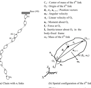
Fig. 1 Conceptualisation of a chain as a multibody system
with the existing results are presented in Sect.3. Some insights into the performance of the proposed algorithm are presented in Sects. 4and5, whereas conclusions are provided in Sect.6.
2 Mathematical formulation
Figure1shows the schematic of a chain as a system of a number of rigid links. Here, the chain is considered to have spatial motion rather than planar, as studied in [6,12,15,16]. The #kth link in a chain is connected to the #(k−1)th link by a one-, two- or three-DOF joint, say, revolute, prismatic, universal, or spherical, depending on the application. Link #0 is the base link which may be fixed or have some prescribed motion. As the chain may contain multi-DOF joints, the total number of DOF of the chain, denoted by n, may be different from the total number of links (denoted bynl) in a chain.
here for the sake of completeness of the paper. The equations pertaining to the kinematics and dynamics are represented with respect to the origin of the local coordinate system at-tached to the link.
The NE equations of motion for the #kth link (Fig. 1(b)) moving freely in the 3-dimensional Cartesian space are written in the matrix form [23] as
Mk˙tk+kMkEktk=wk, (1)
whereMk,k, andEkare the 6×6 extended mass, angular velocity, and coupling matrices,
respectively;tkandwkrepresent twist of, and wrench acting on the #kth link, respectively.
They are defined as
skew-symmetric matrices associated with the vectorsdkandωk, respectively; “O” and “1”
represent null and identity matrices of compatible dimensions, respectively. Fornllinks, the
uncoupled NE equations of motion can be assembled as
M˙t+MEt=w, wherew=wE+wC, (3)
whereM,, andEstand for the 6nl×6nlgeneralised extended mass, the angular velocity,
and the coupling matrices [23], respectively. Moreover,wEandwCare the 6n
l-dimensional
vectors of external/working wrench and constraint wrench, respectively.
2.1 Velocity constraints
The velocity constraints leading to the expression of the DeNOC matrices are obtained next. In contrast to [29], where the joints had only one-DOF, here the #kth link is connected to the #(k−1)th link by either single- or multi-DOF jointk. The number of joint variables associated with thekth joint is denoted byzk. Next, the twist associated with the links #k
and #(k−1)connected by a multi-DOF jointkis given by [30]
tk=Ak,k−1tk−1+Pkθ˙k. (4)
In Eq. (4), Ak,k−1 is the 6×6 twist-propagation matrix [30];Pk is the 6×zk
motion-propagation matrix, andθ˙kis thezk-dimensional joint rate vector. They are defined as
Ak,k−1≡
vector [30] corresponding to the motion about or along thejth axis of thekth multi-DOF joint. The vectors of the generalised twist and the generalised joint-rates for thenllinks of
a serial chain are defined, respectively, as
t≡
twist,t, for the serial chain is obtained as
t=Nq˙. (7a)
In Eq. (7a), the 6nl×nmatrixNrepresents the velocity transformation matrix, which
relates the generalised twist with the generalised joint rate. It may be factored as
N=NlNd, (7b)
whereNlis the 6nl×6nl matrix whileNd is the 6nl×nmatrix. The matricesNlandNd
are the decoupled form of the velocity transformation matrix or simply the DeNOC matri-ces [23] given by
As the net power due to constraint moments and forces, i.e., wrenches, is zero, the vector of constraint forces and moments is orthogonal to the columns ofN. As a result, premultiplying Eq. (3) byNT nullifies the constraint wrenches [29] leading to the equations involving the
“external” wrenches alone, i.e.,
Iq¨+Cq˙=τ. (9)
In Eq. (9), the expressions for then×nGeneralised Inertia Matrix (GIM),I, is given
by
I≡NT
dMN˜ d, (10a)
whereM˜ ≡NT
lMNlis the 6nl×6nl matrix comprising of the 6×6 composite-mass
ma-trices [23]. Moreover, then×nConvective Inertia Matrix (CIM),C, can be expressed in terms of the DeNOC matrices and their time derivatives as
C≡NTd(Ml˜ + ˜Mw+ ˜Me)Nd, (10b)
in whichM˜l≡NTlMN˙l,M˜w≡ ˜M, andM˜e≡NTlMENl. Note that the time derivative of Nd, i.e.,Nd˙ , is equal toNd, which is used in writing the expressions of CIMCof Eq. (10b).
Finally, then-dimensional vector of the generalised external forces (e.g., externally applied forces/moments, forces/moments resisting the motion, etc.),τ, has the following expression:
where the 6nl-dimensional vector,w˜E, is expressed as
˜
wE≡NTlw E
. (10d)
Equation (9) represents the independent set of constrained equations of motion for the chain at hand with multi-DOF joints.
In the forward dynamics, the joint accelerations,q, is typically obtained using GE or¨
Cholesky decomposition [25], which requires O(n3) calculations—n being the
degrees-of-freedom (DOF) of the chain under study. Hence, the solution becomes computationally expensive for large n. However, recursiveO(n) algorithms are popular for this purpose due to their computational efficiency and numerical stability [31]. The algorithm used in this paper, i.e., using ReDySim, is based on theUDUT
decomposition [26,27] of the GIM which uses Reverse Gaussian Elimination or RGE. This leads to a recursiveO(n)forward dynamics algorithm, which is summarised in AppendixA.1for the sake of completeness.
3 Numerical simulations
Several numerical simulations were carried out on chains with a wide range of DOF. Each chain is specified by the types of links and joints, the number of links, and the total length of the chain. For example, in RE-Rnl-Liand RE-Unl-Li, RE refers to the fact that the links of the chain are made of “rigid elements.” The term R or U signifies that the joints are either “revolute” or “universal,” andnlrepresents the number of links. Likewise, Lidenotes the total length of the chain in meters. Note that an RE-Rnl-Li chain hasnl-DOF, while RE-Unl-Li is a 2nl-DOF system because a universal joint has two-DOF in contrast to the revolute joint, which has only one-DOF. The numerical integrations were performed using MATLAB’s in-built ODE solver ODE45, which is based on an adaptive fourth–fifth-order Runge–Kutta method. All simulations were carried out with relative and absolute tolerances of 10−4and 10−6, respectively, unless otherwise stated. The numerical results obtained are
presented in the following subsections.
3.1 Validation of ReDySim with experimental and numerical results
In this subsection, the ReDySim algorithm has been validated against experimental and numerical results available in existing literature [12] on the planar chains. For the spatial chains, the results have been compared with those generated using the commercial software RecurDyn [24], as similar experimental results could not be found in the literature. The algorithm is then applied to simulate and analyse a wide range of spatial chains.
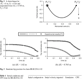
Various configurations of RE-R229-L1.02, i.e., a 1.02 m long chain with a total mass of 0.0208 kg and 229 identical links, connected by only revolute joints were analysed experi-mentally as well as numerically in [12], where the main objective was to study the effect of initial horizontal separation on the behaviour of the chain tip motion.
Let a chain of lengthLbe held between two points (X1,Y1) and (X2,Y2), as shown
in Fig.2. The horizontal and vertical separations between the two points are denoted by X=X2−X1andY =Y2−Y1, respectively. Two configurations, as defined in Table1,
were used to validate the algorithm with the reported experimental and numerical results in [12]. The initial joint angles of the chain were obtained by considering the chain to form a catenary while in static equilibrium [32].
Fig. 2 A chain hinged at (X1=0 m,Y1=0 m) and suspended from (X2=0.765 m,
Y2=0 m)
Fig. 3 Simulated tip position for chain RE-R229-L1.02
Table 1 Initial conditions and CPU time for RE-R229-L1.02 [12]
Initial configuration of the chain (m) (Y=0)
Initial velocity imparted to the system (m/s)
Simulation time (s)
CPU time (s)
X=1.02 0.0 0.5 31.4
X=0.765 0.0 0.5 28.5
algorithm match with those obtained experimentally in [12]. Interestingly, the CPU time required to simulate the chain decreases with decreasingX, as shown in Table1. Small
Ximplies that the chain is closer to its most stable configuration, i.e., vertical. This makes the system of equations less stiff [33], and hence, the solution is attained faster.
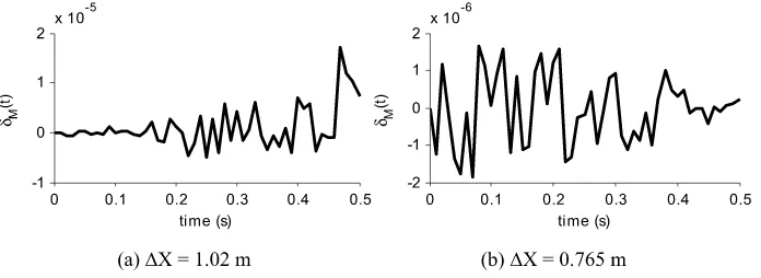
Figure4shows comparison of simulated tip velocity and acceleration magnitude with the same obtained numerically in [12]. The results are in close match with those obtained in [12]. The peak velocity and acceleration magnitude decrease with smallerX. Figure5 shows the change in total instantaneous energy per unit mass of the chain defined as
δM(t )=
E(t )−E(0)
M , (11)
Fig. 4 Simulated tip velocity and acceleration magnitudes for chain RE-R229-L1.02
Fig. 5 Change in total instantaneous energy per unit mass,δM(t ), for RE-R229-L1.02
the two configurations of RE-R229-L1.02, respectively, which demonstrates the accuracy of the solution.
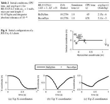
Analysis of spatial motion of chains was performed next by replacing the revolute joints with universal joints having axes of rotations orthogonal to the length of the link elements. Figure6shows the initial horizontal configuration of RE-Unl-L1 chain with gravitational field acting in the negativeY-direction and an initial out-of-plane velocity,ωY0, applied to all the links aboutY0. Each link of (Li/nl) m long has a uniform circular cross-section of diameter 0.10 m and mass per unit length as 61.65 kg/m for all the simulations performed. The initial horizontal configuration of the chain corresponds to zero potential energy. All chains have initial energy resulting out of the nonzero kinetic energy due to initial angular velocity of the chain.
As shown in Table2, spatial motion of RE-U125-L1 with 250 degrees-of-freedom (DOF) due to the presence of 2-DOF universal joints, denoted by U, was simulated by imparting
ωY0=1.0 rad/s in both ReDySim and RecurDyn [24] with common absolute tolerances
of 10−6. The results of the tip position obtained using ReDySim are in close match with
Table 2 Initial conditions, CPU time, and avg|δM(t )|for
RE-U125-L1 withωY0=1 rad/s, mass per unit length=
61.65 kg/m and integrator absolute tolerance of 10−6
RE-U125-L1 (X=1,Y=0)
E(0)
(Joules)
Simulation time (s)
CPU time (s)
avg|δM(t )|
(Joule/kg)
ReDySim 10.2756 1.0 65 2.15e−6 RecurDyn 10.2756 1.0 678 3.11e−3
Fig. 6 Initial configuration of a RE-Unl-L1 chain
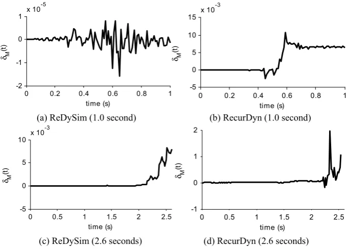
Fig. 7 Simulated tip position of RE-U125-L1
using both RecurDyn and ReDySim, was plotted in Fig.9(a–b). The plots clearly show that in RecurDyn,δM(t ), after 0.45 seconds, is 103times larger than that of ReDySim. As seen from Fig.7, the chain tip reaches its bottommost position at∼0.45 second before moving up, causing large joint accelerations of the order of 100g, which are difficult to capture numerically in an accurate manner. ReDySim took 65 seconds of CPU time to complete the 1.0 second simulation as compared to 678 seconds taken by RecurDyn on a 2 GHz Core2Duo-powered laptop.
Fig. 8 Simulated tip velocity and acceleration magnitude for RE-U125-L1
Fig. 9 Comparison of change in total instantaneous energy per unit mass,δM(t ), using simulation results for ReDySim and RecurDyn for absolute error tolerances of 10−6
3.2 Simulations of moderate- and large-DOF chains using ReDySim
In this section, simulation results for moderate- and large-DOF chains are presented, which were obtained using ReDySim algorithm. Note that Tables3and4show the initial condi-tions of several moderate- and large-DOF chains falling under gravity. The tables also show the simulation time, corresponding CPU time, and the average value of|δM(t )|.
Table 3 Initial conditions, CPU time, and avg|δM(t )|for chains with moderate-DOF (ωY0=1.0 rad/s and
mass per unit length=61.65 kg/m)
Chain specification
Initial configuration of the chain (m) (Y=0)
E(0) (Joules)
Simulation time (s)
CPU time (s)
avg|δM(t )| (Joule/kg)
RE-U125-L1 X=1 10.27 1.0 34.2 2.15e−6
RE-U250-L2 X=2 82.20 1.0 111.5 3.48e−6
RE-U375-L3 X=3 277.44 1.0 201.5 4.68e−6
Table 4 Initial conditions, CPU time, and avg|δM(t )|for chains with large-DOF (ωY0=1.0 rad/s and mass
per unit length=61.65 kg/m)
Chain specification
Initial configuration of the chain (m) (Y=0)
E(0) (Joules)
Simulation time (s)
CPU time (s)
avg|δM(t )| (Joule/kg)
RE-U750-L6 X=6 2,219.53 2.0 1330 8.37e−6
RE-U1250-L10 X=10 10,275.62 2.0 2803 1.35e−5
RE-U3750-L30 X=30 277,441.90 2.0 12194 3.71e−5
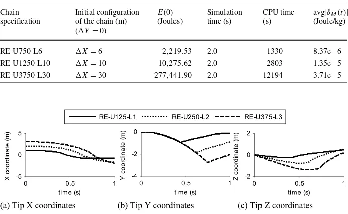
Fig. 10 Simulated tip position of moderate-DOF chains using ReDySim
worth noting that the acceleration increases with an increase in the length of the chain. As a result, the governing equations of motion become stiff and an adaptive solver (e.g., ODE45 in MATLAB) requires smaller step sizes to achieve acceptable error tolerances. Hence, the peak value of the acceleration cannot be captured if the results are sampled too sparsely. The simulation results for the large-DOF chains corroborate the above observation. The peak value of acceleration could not be captured as the results were sampled after every 0.05 seconds. Nevertheless, when acceleration for RE-U-750-L6 (1500-DOF) was obtained using results generated at all the steps (71,488 steps were required by ODE45 for 2.0 seconds of simulation time), the peak value of 5335 m/s2was observed at 1.036 seconds. Note that
Fig.13(b) shows lower values due to the sparse sampling.
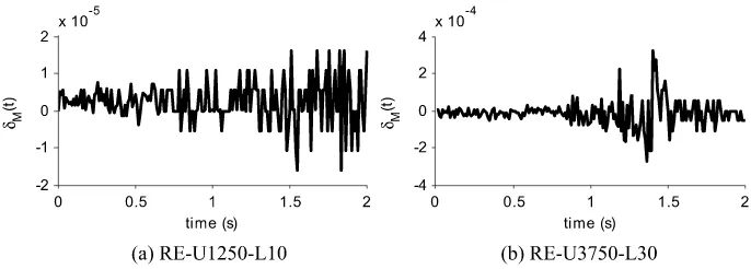
The change in total instantaneous energy per unit mass for chains RE-U1250-L10 (2500-DOF) and RE-U3750-L30 (7500-(2500-DOF) was of O(10−5) and O(10−4), respectively, as
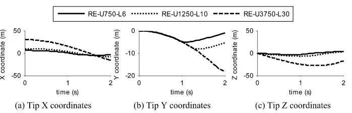
Fig. 11 Simulated tip position of large-DOF chains using ReDySim
Fig. 12 Simulated tip velocity and acceleration magnitude for moderate-DOF chains using ReDySim
Fig. 13 Simulated tip velocity and acceleration magnitude for large-DOF chains using ReDySim
3.3 Simulation of huge-DOF chains using ReDySim
Fig. 14 Change in total instantaneous energy per unit mass,δM(t ), for large-DOF chains using ReDySim
Table 5 Initial conditions, CPU time, and avg|δM(t )|for chains with huge-DOF (ωY
0=1.0 rad/s and mass
per unit length=61.65 kg/m)
Chain specification Initial configuration of the chain (m) (Y=0)
E(0)
(Joules)
Simulation time (s)
CPU time (s)
avg|δM(t )| (Joule/kg)
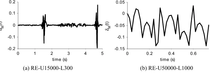
RE-U5000-L100 X=100 1.027e+7 5.0 35848 1.14e−3 RE-U7500-L150 X=150 3.468e+7 5.0 71242 2.13e−3 RE-U10000-L200 X=200 8.220e+7 5.0 126905 3.46e−3 RE-U15000-L300 X=300 2.774e+8 5.0 230598 9.50e−3 RE-U50000-L1000 X=1,000 1.027e+10 0.75 365352 5.72e−2
Fig. 15 Simulated tip position for huge-DOF chains using ReDySim
Figures15(a–c) show theX,Y, andZcoordinates of the tip, while Figs.16(a–b) depict the magnitudes of the tip velocity and acceleration. As stated earlier, the tip acceleration magnitude at the bottommost position is higher for a longer chain. Since the results were sampled every 0.05 seconds, the finer variations in tip velocity and acceleration magnitude are not captured.
Fig. 16 Simulated tip velocity and acceleration magnitude for huge-DOF chains
Fig. 17 Change in total instantaneous energy per unit mass,δM(t ), for huge-DOF chains using ReDySim
The simulation of RE-U50000-L1000 could not proceed beyond 0.75 seconds due to the limitation of the computer’s memory.
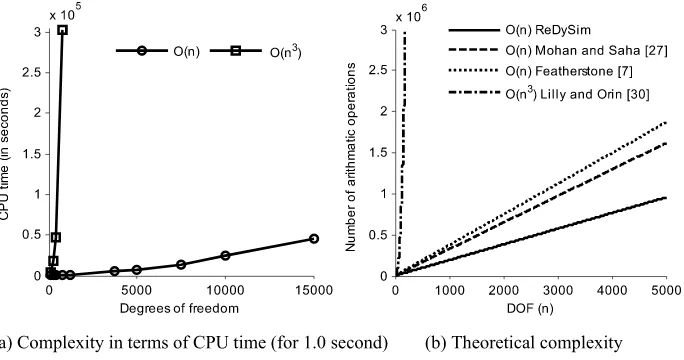
4 Efficiency, accuracy, and numerical stability of ReDySim
Analysis of chains based on the solution of joint accelerations using an algorithm of
O(n3)—nbeing the degrees-of-freedom (DOF) of the system at hand—complexity is com-mon in literature [6,12]. Hence, simulations of several moderate- and large-DOF systems were also carried out using a classical GE-basedO(n3)solver developed in-house. Note that a more common technique to solve for the joint accelerations is to decompose the symmetric positive definite GIM of Eq. (10a) using Cholesky decomposition [25] followed by forward and backward substitutions. This approach also hasO(n3)complexity. For the GIM, the GE-based decomposition is equivalent to the Cholesky decomposition without the necessity of evaluating the square-root terms [25]. Hence, the GE-based decomposition of the GIM was preferred for the in-house development ofO(n3)algorithm. The results were then compared with those obtained from ReDySim, which uses an analytical Reverse GE (RGE)-based de-composition [26,27]. This leads to anO(n)algorithm. The comparisons were then carried out in terms of efficiency, accuracy, and numerical stability.
Table 6 Comparison of ReDySim with GE-basedO(n3)solver with regard to efficiency (ωY0=1.0 rad/s)
Chain specification
Initial configuration of the chain (m) (Y=0)
E(0)
(Joules)
Simulation time (s)
CPU time for
O(n3)(s)
CPU time for ReDySim (s)
RE-U125-L1 X=1 10.276 1.0 3,399 34.2 RE-U250-L2 X=2 82.205 1.0 18,473 111.5 RE-U375-L3 X=3 277.442 1.0 47,697 201.5 RE-U750-L6 X=6 2,219.535 1.0 303,134 665.1
Table 7 Detailed operation count for various forward dynamics algorithms [23]
Algorithms Computational complexity
Multiplications/divisions Additions/subtractions
ReDySim 135nr+99nu+87ns−116 131nr+92nu+7923ns−123 Mohan and Saha [31] 173n−128 150n−133
Featherstone [7] 199n−198 174n−173
Lilly and Orin [34] 16n3+1032n2+4013n−51 16n3+7n2+5056n−51
Note:n=nr+nu+ns, wherenr,nu, andnsare the total DOF associated with all revolute, universal, and spherical joints, respectively
Fig. 18 Comparison of complexities using ReDySim, an in-houseO(n3), and otherO(n)algorithms
also reflected in Table7and Fig.18(b), where theoretical complexities reported in the liter-ature are compared with that of ReDySim. In terms of computational complexity, ReDySim with special treatment of multi-DOF joint [30] performs better thanO(n3)and otherO(n)
algorithms available in the literature, e.g., in [7,31,34].
with 100,000-DOF. This shows the capability of the solver in simulating such huge systems accurately.
Numerical stability of the algorithm is another important issue, which directly affects the accuracy of the results. As defined in [35], an algorithm is called numerically stable if it is stable in the mixed forward-backward error sense. Numerical stability mainly depends on the method of solving the problem rather than the order of complexity of the solver. It will be shown in the next section that the algorithm in ReDySim based on RGE is more stable than the algorithm based on GE.
5 Numerical issues with simulation of chains
In this section, some issues related to simulation of long chains are discussed, such as, ill-conditioning and other characteristics of the GIM of Eq. (10a) including a comparison of the GE- and RGE-based methods of solving joint accelerations.
5.1 Ill-conditioning of the GIM
The equations of motion obtained in Eq. (9) are used to solve for the joint angles and ve-locities. The solution involves: (1) computation of the joint accelerations, and (2) numerical integration of the same for the given initial values of position and velocity. Computation of the joint accelerations, denoted byq¨, is given by
¨
q=I−1ϕ, whereϕ=τ−Cq˙. (12)
To computeq¨from Eq. (12), one can decompose the GIM asLUorLLT [25] using GE
or Cholesky decomposition, respectively, followed by forward and backward substitutions. The matricesLandUare the lower and upper triangular matrices, respectively. However, when the GIM becomes ill-conditioned, small perturbations in the system of equations can produce relatively large changes in the numerical solutions. Ill-conditioning of a matrix is defined as its closeness to singularity [25]. If the system represented in Eq. (12) satisfies
(q¨+δq¨)=I−1(ϕ+δϕ), (13)
the relative deviation in computation of the joint accelerations is given by
δq¨ ¨q ≤κ(I)
δϕ
ϕ, (14)
whereκ(I)= I−1IandIrepresents the norm of the GIM. The termκ(I)is defined as the condition number of the GIM, which determines the scale factor by which the relative change or deviation inq¨ is magnified. If the condition number of the GIM is very high, it is ill-conditioned or close to singular. TheL2-norm [25] gives the condition number of the GIM, denoted byκ2(I), as
κ2(I)= σmax(I) σmin(I)
, (15)
whereσmax(·) andσmin(·) are the maximum and minimum singular values of a matrix. As the GIM is symmetric and positive definite, its singular values are equal to the corresponding eigenvalues, and Eq. (15) can be rewritten as
κ2(I)= λmax
whereλmaxandλminare the highest and smallest eigenvalues of the GIM,I.
As discussed in the Introduction, the GIM of a serial-chain withn-DOF has condition
number anywhere betweenO(n)andO(4n4)[7]. Hence, with an increase inn, there can be
loss of accuracy in the computation of the joint accelerations.
5.2 Investigation of the accuracy of the ReDySim solver
In order to investigate why ReDySim solver produced numerically more accurate results, a comparative study of three different methods to calculate the joint accelerations was carried out. They are:
1. Gaussian Elimination(Numerical) or GE-N: Using GE [25], annihilations of the
below-diagonal elements of the GIM given by Eq. (10a) were carried out starting from the first
column toward the last column to obtain an upper triangular matrix. This is also referred to as the sweep out phase. Typically, such procedure is numerical in nature leading to
O(n3/6)complexity. For the computation of the joint accelerations using Eq. (12),
for-ward and backfor-ward substitutions were performed, requiringO(n2)operations. Hence,
the overall computational complexity is said to beO(n3). The method is represented by
GE-N for future references to emphasise the fact that it is a purely numerical procedure. 2. Reverse Gaussian Elimination (Numerical) or RGE-N: In contrast to the classical
GE [25] mentioned above, in RGE, as introduced in [26,27], annihilations of the
above-diagonal elements started from the last column and proceeded toward the first column to convert the GIM into a lower triangular matrix. The steps of the RGE were performed nu-merically having the same number of operations as GE-N. The term RGE-N will be used for future references to emphasise that it is a numerical procedure as well. For the com-putation of the joint accelerations, backward and forward substitutions were performed,
leading to an overall computational complexity ofO(n3).
3. Reverse Gaussian Elimination(Analytical) or RGE-A: This method is same as explained in item 2. However, the steps of annihilations and substitutions were performed analyti-cally, without using any numerical values for the link lengths or masses, as explained in
[26,27]. Such steps, as outlined in AppendixA.1, lead to a set of recursive expressions
withO(n)computational complexity. The abbreviation RGE-A will be used for future
references, where “A” is used to emphasise that the steps were performed analytically. The RGE-A method is used in ReDySim.
The joint accelerations obtained using all the above three methods were then numerically integrated using the ODE45 integrator of MATLAB to yield joint velocities and angles, which are further used to calculate the tip positions and velocities.
The dynamical systems used for the study here are 3- and 10-link chains with identical
link length of 1.0 m each, cross-sectional radius of 0.02 m, and 7025 kg/m3material density,
falling under gravity. Since all the schemes performed well at the double precision accuracy,
the floating point accuracy was reduced to 10−3and 10−5, so as to accentuate the
numer-ical errors, leading to clear differentiation between the results generated by the different methods. The 3-link chain was simulated for 5.0 simulation seconds with a floating point
accuracy of 10−3, and the 10-link chain was simulated for 3.0 simulation seconds with 10−5
floating point accuracy.
Table8shows the number of steps required by the adaptive integrator ODE45 of
Table 8 CPU time and number of steps for simulation of 3- and 10-link chains
3-link chain with accuracy of 10−3 10-link chain with accuracy of 10−5 Simulation
time (s)
No. of steps
CPU time (s)
Simulation time (s)
No. of steps
CPU time (s)
GE-N 5.0 618 2.89 3.0 4723 236.2
RGE-N 5.0 231 1.24 3.0 196 12.6
RGE-A 5.0 134 1.48 3.0 177 5.3
Fig. 19 Change in total instantaneous energy per unit mass,δM(t ), using GE-N, RGE-N, and RGE-A
Table 9 Solution ofq¨(0)with
double precision accuracy I(0) ϕ(0) q¨(0)
79.4535 41.1985 11.7714 41.1985 23.5428 7.3574 11.7714 7.3574 2.9435
−194.8533
−86.6015
−21.6504
−6.2242
7.9198
−2.2602
κ2(I(0))=309.2300
Figure19(a–b) show the change in total instantaneous energy per unit mass. It is clearly evident that RN-, and RA-based solvers perform significantly better than the GE-N-based solver, while RGE-A-based solver (used in ReDySim) performs even better than RGE-N-based solver.
5.3 Numerical stability of GE-N, RGE-N, and RGE-A
In order to test the stability of GE-N-, RGE-N-, and RGE-A-based solvers described in Sect.5.2, the GIMIand the vectorϕof Eq. (12) for a 3-link planar chain are considered.
The numerical values ofIandϕcorresponding to the initial horizontal configuration of the
chain, i.e., whenq(0)=0, denoted byI(0)andϕ(0), respectively, are shown in Table9. The
joint accelerations, i.e.,q(0), were then obtained using MATLAB’s command “I(0)¨ \ϕ(0)”
with double precision accuracy. These results were considered as “correct” and were used as benchmarks for the comparisons performed.
Table 10 Comparison of GE-N, RGE-N, and RGE-A with variable floating point round off
Note: NaN denotes “Not a Number”
in Table10. The table shows the joint accelerations obtained using the corresponding solvers
and the percentage deviations relative toq(¨ 0), as given in Table9. For a given floating point accuracy, the percentage error, denoted byδq¨ is defined as
δq¨≡ round-offs, andq¨i(0)is the solution obtained using MATLAB with double precision accu-racy. Here, the absolute deviation is avoided to emphasise on howq¨iF(0)varies aroundq¨i(0).
It is evident from Table10that the percentage deviation is lower for the RGE-A-based solver
while the GE-N-based solver showed higher deviations. As the floating point accuracy of the computing system was made higher, the solution for joint accelerations obtained from the
RGE-N- and RGE-A-based solvers converged faster to the desired solutionq(¨ 0)than the
GE-N-based solver.
Note that the solution of Eq. (12), which is linear in the unknownq¨, using GE-N- or RGE-N- or RGE-A-based solvers essentially consists of two phases, namely, annihilations or sweep-out and substitutions [36]. The sweep-out phase of GE-N starts with the first element
Table 11 Variation of the percentage error inq¨1andq¨nl with the number of links (floating point accuracy
=10−7)
Links (nl) Condition number
of GIM,I
GE-N RGE-A δq¨1[during
sweep-out]
δ¨qnl [during
substitution]
δ¨qnl [during
sweep-out]
δq¨1[during
substitution]
5 2,708.4 0.0031645 1.4148 −0.0006998 1.2319e−5 10 4.3473e+4 0.0051407 −1,928.4 0.26676 −5.6754e−6 20 6.6955e+5 −0.58922 −4.6793e+10 7.1426e+5 −5.6762e−6 40 1.0371e+7 1.1572 5.4647e+13 −6.296e+8 −5.6744e−6 60 5.1814e+7 12.779 −4.7533e+13 −1.1474e+8 −5.6842e−6 80 1.6260e+8 11.337 −2.6018e+15 −6.8846e+8 −5.6717e−6 100 3.9523e+8 −272.25 −5.2965e+15 1.7183e+8 −5.6563e−6
starts with the last element of the last column, i.e.,i33=2.9435. Each equation in Eq. (12) represents a plane, and these three planes intersect at the required solution q¨, as shown in Fig. 20(a). As explained in [36] and outlined in Appendix A.2, the GE-N transforms the GIM,Iof Eq. (10a), to a upper triangular matrix, denoted withU, reducing the set of algebraic equations forIq¨=ϕtoUq¨= ¯ϕ, whereϕ¯is related toϕasϕ¯=L−1ϕin whichL−1 is the resulting matrix representing the sweep-out phase. Geometrically,Uq¨= ¯ϕrepresents the two planes given by the last two equations ofIq¨=ϕrotated about the solution point, as depicted in Fig.20(b). If these planes are nearly orthogonal to each other, then the accuracy of the solution in the following substitution phase, i.e.,Uq¨= ¯ϕ, is better, as they are less sensitive to errors in the right hand side values. This aspect is explained in AppendixA.2. On the other hand, RGE-N or RGE-A which transforms the GIM, matrixIof Eq. (10a), to a lower triangular matrix, denoted byL′, reducing the set of algebraic equationsIq¨=ϕto
L′q¨=ϕ′, whereϕ′can be related toϕasϕ′=(U′)−1
ϕin which matrix(U′)−1represents the resulting matrix of the sweep-out phase using RGE. The equationL′q¨=ϕ′represents the first two planes ofIq¨=ϕrotated about the solution point, as depicted in Fig.20(c). Comparing Figs.20(b) and20(c), it may be seen that the said planes after N or RGE-A are closer to being mutually orthogonal, than in the case of GE-N. Hence, the substitution phase of RGE-N or RGE-A would yield better solutions than GE-N.
To consolidate the above observations, numerical experiments were carried out on a va-riety of single-DOF joint chains (nl=n) at a fixed initial configuration, i.e.,q(0)=0. The joint accelerations were computed using GE-N- and RGE-A-based solvers, fort=0 second and floating point accuracy of 10−7, in order to study the propagation of errors in substitu-tion phase. It was assumed that some error has already been introduced during the sweep-out phases inq¨1andqn¨l, for GE-N and RGE-A, respectively. The resulting differences in solu-tions ofqn¨ l andq¨1due to substitution phases in GE-N and RGE-A, respectively, are shown in Table11. It can be seen from Table11that with an error inq¨1, i.e.,−272.25 % for 100-link chain, during the sweep-out phase, the error in the solution ofq¨nl is magnified to the O(1015). In case of RGE-A, however, even if there is an error ofO(108)inqn¨
6 Conclusions
This paper investigated the dynamic behaviour of serial chains with degrees-of-freedom up to 100,000. Simulations were performed using Recursive Dynamics Simulator (ReDySim) developed for general tree-type systems. Such large-DOF systems were never previously re-ported in literature. Moreover, such systems failed to produce any results using commercial software like RecurDyn. The accuracy, stability, and efficiency, which are important for long serial-chain systems as those qualities deteriorate with the increasing number of links,nl, were proven nearly insensitive when ReDySim algorithm was used. These observations es-tablished the viability of solution of a large number of engineering problems with high-DOF using ReDySim.
Acknowledgements The authors acknowledge the Naren Gupta Chair Professor fund of the last author at IIT Delhi, which was used to support the second author to conduct this research. Anonymous reviewers are also thanked for their constructive comments.
Appendix
A.1 RecursiveO(n)forward dynamics
In this section, outline of the recursiveO(n)forward dynamics algorithm implemented in Recursive Dynamics Simulator (ReDySim) solver and used for the simulation of chains with large-DOF are presented. The algorithm is based on theUDUT decomposition of the GIM [27] using analytical Reverse Gaussian Elimination, denoted by RGE-A. The forward dynamics essentially involves the calculation of joint accelerations from Eq. (9) as
¨
q=I−1ϕ, whereϕ=τ−Cq˙. (A.1)
Using the decompositionI=UDUT, the equations of motion, Eq. (A.1), are rewritten as follows:
UDUTq¨=ϕ, (A.2)
Table 12 Forward dynamic algorithm [23]
Backward recursion:Computation ofϕˆandϕ˜
For link #k (k=nl, . . . ,1) ϕˆk=ϕk−PTkη˜k, whereη˜k=ATk+1,kηk+1
andηk+1=k+1ϕˆk+1+ ˜ηk+1 ˜
ϕk= ˆI −1 k ϕˆk Forward recursion:Computation ofq¨fromUTq¨= ˜ϕ
For link #k (k=1, . . . , nl) θ¨k= ˜ϕk−Tkμ˜k, whereμ˜k=Ak,k−1μk−1
andμk−1=Pk−1θ¨k−1+ ˜μk−1
In Eq. (A.5), the 6×6 matrix Mˆk contains the mass and inertia properties of the
articulated-body #k[23]. The matrixMˆkis computed as follows:
ˆ
Mk=Mk+ATk+1,kMˆk+1,k+1Ak+1,k, (A.6)
whereMˆn≡Mn. Moreover, the 6×6 matrixMˆk+1,k+1in Eq. (A.6) is obtained as
ˆ
Mk+1,k+1= ˆMk+1− ˆk+1Tk+1. (A.7)
The joint accelerations are then obtained using three sets of linear algebraic equations, namely
(i) Uϕˆ=ϕ, whereϕˆ≡DUTq¨,
(ii) Dϕ˜= ˆϕ, whereϕ˜≡UTq¨, (A.8)
(iii) UTq¨= ˜ϕ.
From Eq. (A.8), the recursive algorithm, comprising of the backward recursions arising from steps (i) and (ii), and forward recursions, arising from step (iii), is summarised in Ta-ble12. It is assumed in Table12that the vectorϕ, comprised of the external joint torques and those due to Coriolis and centripetal accelerations, is calculated using anO(n)inverse dynamic algorithm after settingθ¨=0, as shown in [29]. The effect of gravity can be taken into consideration during the inverse dynamics calculations by adding the gravitational ac-celeration vector into the twist-rate of the first link. Table12explains the steps involved in forward dynamic calculations.
A.2 Geometric interpretations of GE and RGE
After GE-N, which is denoted here with simply GE as no numerical aspect is emphasised, the GIM of Eq. (10a) is converted to an equivalent upper triangular matrix during the an-nihilations or sweep-out phase, whereas the solution of the joint accelerations is obtained using backward substitution as
GE: Iq¨=ϕ Phase 1⇒ Uq¨= ¯ϕ Phase 2⇒ q¨=U−1ϕ¯. (A.9)
Table 13 Condition number of the matrices resulting out GE and RGE
are shown in Table13. On the contrary, in RGE-N or RGE-A, which are denoted here by RGE only because no numerical or analytical aspect is emphasised, the GIM of Eq. (10a) is converted into an equivalent lower triangular matrix during the sweep-out phase, and the solution of the joint accelerations are obtained using forward substitution as
RGE: Iq¨=ϕ Phase 1⇒ L′q¨=ϕ′ Phase 2⇒ q¨=L′−1ϕ′. (A.10)
In RGE, the matrix representing multipliers of the sweep-out phase is an upper triangular matrix such thatI=U′L′. The matricesU′
andL′and their condition numbers are also given in Table13.
It can be seen from Table13that the condition number ofLafter GE isκ2(L)=2.17,
which ensures the accuracy of the sweep-out phase. However, the condition number ofU,
κ2(U)=223.11, makes backward substitution phase inaccurate or sensitive to small error in
the right-hand side, as shown in Table9. On the other hand, in RGE,κ2(U′)=21.46 while κ2(L′)=15.15. Hence, both the phases have low sensitivity to deviations in the right-hand
sides, thereby, giving better solution to the system of linear equations.
This above fact was also supported in [36], where it was shown geometrically that the use of partial pivoting to achieve stability in sweep-out phase may reorient the planes such that it makes substitution phase highly inaccurate. Hence, geometric analysis of both GE and RGE was performed. Figure20(a–c) show the planes of the original system,Iq¨=ϕ, and reoriented systemsUq¨= ¯ϕdue to GE of the GIM andL′q¨=ϕ′due to RGE. Figure20(a) shows that the original system is poorly oriented as the angles between them are small. The GE does not make the situation better as planes 2 and 3 are still poorly oriented, as shown in Fig.20(b). As GE starts backward substitution with calculation ofq¨3, small deviation in
¨
q3 (orientation of plane 3) causes large changes inq¨2and q¨1. On the other hand, RGE of
the GIM, as shown in Fig.20(c), makes the orientation of the plane favourable for forward substitution as the angle between the planes is higher. Hence, small deviations inq¨1do not
result into large changes inq¨2andq¨3.
References
1. Spong, M.W., Vidyasagar, M.: Robot Dynamics and Control. Wiley, New York (1989)
2. Nakamura, Y.: Advanced Robotics: Redundancy and Optimization. Addison Wesley, Reading (1991) 3. Vold, H.I., Karlen, J.P., Thompson, J.M., Farrell, J.D., Eismann, P.H.: A 17 degree of freedom
anthro-pomorphic manipulator. In: Proceedings of NASA Conference on Space Telerobotics, vol. 1, pp. 19–28 (1989)
5. Gerstmayr, J., Schoberl, J.: A 3D finite element method for flexible multibody systems. Multibody Syst. Dyn.15, 309–324 (2006)
6. Fritzkowski, P., Kami´nski, H.: Dynamics of a rope as a rigid multibody system. J. Mech. Mater. Struct. 3(6), 1059–1075 (2008)
7. Featherstone, R.: An empirical study of the joint space inertia matrix. Int. J. Robot. Res.23(9), 859–871 (2005)
8. Featherstone, R.: A divide-and-conquer articulated body algorithm for parallelO(log(n))calculation of rigid body dynamics. Part 2: Trees, loops, and accuracy. Int. J. Robot. Res.18, 876–892 (1999) 9. Yamane, K., Nakamura, Y.: ParallelO(logN )algorithm for dynamics simulation of humanoid robots.
In: 6th IEEE-RAS International Conference on Humanoid Robots (2006)
10. Malczyk, P., Fraczek, J.: Cluster computing of mechanisms dynamics using recursive formulation. Multi-body Syst. Dyn.20(2), 177–196 (2008)
11. Ascher, U.M., Pai, D.K., Cloutier, B.P.: Forward dynamics elimination methods, and formulation stiff-ness in robot simulation. Int. J. Robot. Res.16(6), 749–758 (1997)
12. Tomaszewski, W., Pieranski, P., Geminard, J.: The motion of a freely falling chain tip. Am. J. Phys. 74(9), 776–783 (2006)
13. Aglietti, G.: Dynamic response of a high-altitude tethered balloon system. J. Aircr.46(6), 2032–2040 (2009)
14. Calkin, M.G., March, R.H.: The dynamics of a falling chain: I. Am. J. Phys.57, 154–157 (1989) 15. Fritzkowski, P., Kami´nski, H.: Dynamics of a rope modelled as a discrete system with extensible
mem-bers. Comput. Mech.44, 473–480 (2009)
16. Fritzkowski, P., Kami´nski, H.: Dynamics of a rope modelled as a multi-body system with elastic joints. Comput. Mech.46(6), 901–909 (2010)
17. Gatti, C., Perkins, N.: Physical and numerical modeling of the dynamic behaviour of a fly line. J. Sound Vib.255(3), 555–577 (2002)
18. Hembree, B., Slegers, N.: Efficient tether dynamic model formulation using recursive rigid-body dynam-ics. Proc. Inst. Mech. Eng., Proc., Part K, J. Multi-Body Dyn.224, 353–363 (2010)
19. Kamman, J., Huston, R.: Multibody dynamics modeling of variable length cable systems. Multibody Syst. Dyn.5, 211–221 (2001)
20. Robson, J.M.: The physics of fly casting. Am. J. Phys.58, 234–240 (1990)
21. Schagerl, M., Steindl, A., Steiner, W., Troger, H.: On the paradox of the free falling folded chain. Acta Mech.125, 155–168 (1997)
22. Wong, C., Yasu, K.: Falling chains. Phys. Rev. Lett.74(6), 490–496 (2006)
23. Shah, S.V., Saha, S.K., Dutt, J.K.: Dynamic of Tree-Type Robotic Systems. Springer, Dordrecht (2013) 24. Function Bay Inc.: RecurDyn, Version 7.4 (2009)
25. Strang, G.: Linear Algebra and Its Applications. Harcourt Brace Jovanovich, San Diego (1998) 26. Saha, S.K.: A decomposition of the manipulator inertia matrix. IEEE Trans. Robot. Autom.13(2), 301–
304 (1997)
27. Saha, S.K.: Analytical expression for the inverted inertia matrix of serial robots. Int. J. Robot. Res.18(1), 116–124 (1999)
28. MathWorks Inc.: MATLAB, Version 7.4, Release 2009a (2009)
29. Saha, S.K.: Dynamics of serial multibody systems using the decoupled natural orthogonal complement matrices. J. Appl. Mech.66, 986–996 (1999)
30. Shah, S.V., Saha, S.K., Dutt, J.K.: Denavit–Hartenberg (DH) parametrization of Euler angles. J. Comput. Nonlinear Dyn.7(2), 1–10 (2012)
31. Mohan, A., Saha, S.K.: A recursive, numerically stable, and efficient algorithm for serial robots. Multi-body Syst. Dyn.17(4), 291–319 (2007)
32. Weisstein, E.W.: Catenary. MathWorld—a Wolfram Web resource. http://mathworld.wolfram.com/ Catenary.html. Accessed 31 March 2012 (2012)
33. Shampine, L.F., Gear, C.W.: A user’s view of solving stiff ordinary differential equations. SIAM Rev. 21(1), 1–17 (1979)
34. Lilly, K.W.: Efficient Dynamic Simulation of Robotic Mechanisms. Kluwer Academic, Boston (1993) 35. Higham, N.J.: Accuracy and Stability of Numerical Algorithms. SIAM, Philadelphia (2002)