Return and Risk: The
Capital-Asset-Pricing
Model (CAPM)
C
H
A
P
T
E
R
1
0
E
XECUTIVE
S
UMMARY
T
he previous chapter achieved two purposes. First, we acquainted you with the history of U.S. capital markets. Second, we presented statistics such as expected return, variance, and standard deviation. Our ultimate goal in the next three chapters is to determine the appropriate discount rate for capital budgeting projects. Because the discount rate on a project is a function of its risk, the discussion in the previous chapter on standard deviation is a neces-sary first step. However, we shall see that standard deviation is not the final word on risk.Our next step is to investigate the relationship between the risk and the return of indi-vidual securities when these securities are part of a large portfolio. This task is taken up in Chapter 10. The actual treatment of the appropriate discount rate for capital budgeting is re-served for Chapter 12.
The crux of the current chapter can be summarized as follows: An individual who holds one security should use expected return as the measure of the security’s return. Standard de-viation or variance is the proper measure of the security’s risk. An individual who holds a diversified portfolio cares about the contributionof each security to the expected return and the risk of the portfolio. It turns out that a security’s expected return is the appropriate meas-ure of the security’s contribution to the expected return on the portfolio. However, neither the security’s variance nor the security’s standard deviation is an appropriate measure of a security’s contribution to the risk of a portfolio. The contribution of a security to the risk of a portfolio is best measured by beta.
10.1
I
NDIVIDUAL
S
ECURITIES
In the first part of Chapter 10 we will examine the characteristics of individual securities. In particular, we will discuss:
1. Expected Return.This is the return that an individual expects a stock to earn over the next period. Of course, because this is only an expectation, the actual return may be either higher or lower. An individual’s expectation may simply be the average return per period a security has earned in the past. Alternatively, it may be based on a detailed analysis of a firm’s prospects, on some computer-based model, or on special (or inside) information.
2. Variance and Standard Deviation.There are many ways to assess the volatility of a security’s return. One of the most common is variance, which is a measure of the squared deviations of a security’s return from its expected return. Standard deviation is the square root of the variance.
this relationship can be restated in terms of the correlation between the two securities. Covariance and correlation are building blocks to an understanding of the beta coefficient.
10.2
E
XPECTED
R
ETURN
, V
ARIANCE
,
AND
C
OVARIANCE
Expected Return and Variance
Suppose financial analysts believe that there are four equally likely states of the economy: depression, recession, normal, and boom times. The returns on the Supertech Company are expected to follow the economy closely, while the returns on the Slowpoke Company are not. The return predictions are as follows:
Supertech Returns Slowpoke Returns
RAt RBt
Depression 20% 5%
Recession 10 20
Normal 30 12
Boom 50 9
Variance can be calculated in four steps. An additional step is needed to calculate standard deviation. (The calculations are presented in Table 10.1.) The steps are:
1. Calculate the expected return:
Supertech:
Slowpoke:
2. For each company, calculate the deviation of each possible return from the company’s expected return given previously. This is presented in the third column of Table 10.1. 3. The deviations we have calculated are indications of the dispersion of returns. However,
because some are positive and some are negative, it is difficult to work with them in this form. For example, if we were to simply add up all the deviations for a single company, we would get zero as the sum.
To make the deviations more meaningful, we multiply each one by itself. Now all the numbers are positive, implying that their sum must be positive as well. The squared deviations are presented in the last column of Table 10.1.
4. For each company, calculate the average squared deviation, which is the variance:1
Supertech:
0.140625 0.005625 0.015625 0.105625
4 !0.066875
0.05 0.200.12 0.09
4 !0.055!5.5%!RB
0.20 0.10 0.30 0.50
4 !0.175!17.5%!RA
1
Slowpoke:
Thus, the variance of Supertech is 0.066875, and the variance of Slowpoke is 0.013225. 5. Calculate standard deviation by taking the square root of the variance:
Supertech:
= 0.2586 = 25.86%
Slowpoke:
= 0.1150 = 11.50%
Algebraically, the formula for variance can be expressed as
Var(R) Expected value of
where is the security’s expected return and R Ris the actual return.
R R2 !0.013225
!0.066875
0.000025!0.021025!0.030625!0.001225
4 0.013225
■
T
A B L E1 0 . 1
Calculating Variance and Standard Deviation(1) (2) (3) (4)
State of Rate of Deviation from Squared Value
Economy Return Expected Return of Deviation
Supertech* (Expected return 0.175) RAt
A look at the four-step calculation for variance makes it clear why it is a measure of the spread of the sample of returns. For each observation, one squares the difference be-tween the actual return and the expected return. One then takes an average of these squared differences. Squaring the differences makes them all positive. If we used the differences be-tween each return and the expected return and then averaged these differences, we would get zero because the returns that were above the mean would cancel the ones below.
However, because the variance is still expressed in squared terms, it is difficult to in-terpret. Standard deviation has a much simpler interpretation, which was provided in Section 9.5. Standard deviation is simply the square root of the variance. The general for-mula for the standard deviation is
SD(R)
Covariance and Correlation
Variance and standard deviation measure the variability of individual stocks. We now wish to measure the relationship between the return on one stock and the return on another. En-ter covarianceand correlation.
Covariance and correlation measure how two random variables are related. We ex-plain these terms by extending the Supertech and Slowpoke example presented earlier in this chapter.
E
XAMPLEWe have already determined the expected returns and standard deviations for both Supertech and Slowpoke. (The expected returns are 0.175 and 0.055 for Supertech and Slowpoke, respectively. The standard deviations are 0.2586 and 0.1150, re-spectively.) In addition, we calculated the deviation of each possible return from the expected return for each firm. Using these data, covariance can be calculated in two steps. An extra step is needed to calculate correlation.
1. For each state of the economy, multiply Supertech’s deviation from its expected return and Slowpoke’s deviation from its expected return together. For exam-ple, Supertech’s rate of return in a depression is 0.20, which is 0.375 ( 0.20 0.175) from its expected return. Slowpoke’s rate of return in a de-pression is 0.05, which is 0.005 (0.05 0.055) from its expected return. Mul-tiplying the two deviations together yields 0.001875 [( 0.375) !( 0.005)].
The actual calculations are given in the last column of Table 10.2.This proce-dure can be written algebraically as
(10.1)
where RAtand RBtare the returns on Supertech and Slowpoke in state t. and are the expected returns on the two securities.
2. Calculate the average value of the four states in the last column. This average is the covariance. That is,2
"
ABCovRA, RB
0.0195
4 0.004875
RB
RA
RAt RA !RBt RB
!VarR
2
Note that we represent the covariance between Supertech and Slowpoke as either Cov(RA, RB) or AB. Equation (10.1) illustrates the intuition of covariance. Suppose Supertech’s return is generally above its average when Slowpoke’s return is above its aver-age, and Supertech’s return is generally below its average when Slowpoke’s return is below its average. This is indicative of a positive dependency or a positive relationship between the two returns. Note that the term in equation (10.1) will be positivein any state where both returns are abovetheir averages. In addition, (10.1) will still be positivein any state where both terms are belowtheir averages. Thus, a positive relationship between the two returns will give rise to a positive value for covariance.
Conversely, suppose Supertech’s return is generally above its average when Slowpoke’s return is below its average, and Supertech’s return is generally below its aver-age when Slowpoke’s return is above its averaver-age. This is indicative of a negative depen-dency or a negative relationship between the two returns. Note that the term in equation (10.1) will be negativein any state where one return is above its average and the other re-turn is below its average. Thus, a negative relationship between the two rere-turns will give rise to a negative value for covariance.
Finally, suppose there is no relation between the two returns. In this case, knowing whether the return on Supertech is above or below its expected return tells us nothing about the return on Slowpoke. In the covariance formula, then, there will be no tendency for the deviations to be positive or negative together. On average, they will tend to offset each other and cancel out, making the covariance zero.
Of course, even if the two returns are unrelated to each other, the covariance formula will not equal zero exactly in any actual history. This is due to sampling error; randomness alone will make the calculation positive or negative. But for a historical sample that is long enough, if the two returns are not related to each other, we should expect the covariance to come close to zero.
■
T
A B L E1 0 . 2
Calculating Covariance and CorrelationDeviation Deviation
State Rate of from Rate of from
of Return of Expected Return of Expected Product of
Economy Supertech Return Slowpoke Return Deviations
RAt RBt
(Expected return (Expected return
0.175) 0.055)
Depression !0.20 !0.375 0.05 !0.005 0.001875
( !0.20 !0.175) ( 0.05 !0.055) ( !0.375 " !0.005)
Recession 0.10 !0.075 0.20 0.145 !0.010875
( !0.075 "0.145)
Normal 0.30 0.125 !0.12 !0.175 !0.021875
( 0.125 " !0.175)
Boom 0.50 0.325 0.09 0.035 0.011375
The covariance formula seems to capture what we are looking for. If the two returns are positively related to each other, they will have a positive covariance, and if they are neg-atively related to each other, the covariance will be negative. Last, and very important, if they are unrelated, the covariance should be zero.
The formula for covariance can be written algebraically as
where and are the expected returns for the two securities, and RAand RBare the actual returns. The ordering of the two variables is unimportant. That is, the covariance of Awith Bis equal to the covariance of Bwith A.This can be stated more formally as Cov(RA,RB) Cov(RB,RA) or AB BA.
The covariance we calculated is !0.004875. A negative number like this implies that the return on one stock is likely to be above its average when the return on the other stock is below its average, and vice versa. However, the size of the number is difficult to inter-pret. Like the variance figure, the covariance is in squared deviation units. Until we can put it in perspective, we don’t know what to make of it.
We solve the problem by computing the correlation:
3. To calculate the correlation, divide the covariance by the standard deviations of both of the two securities. For our example, we have:
(10.2)
where Aand Bare the standard deviations of Supertech and Slowpoke, respectively. Note that we represent the correlation between Supertech and Slowpoke either as Corr(RA,RB) or
"AB. As with covariance, the ordering of the two variables is unimportant. That is, the corre-lation of Awith Bis equal to the correlation of Bwith A.More formally, Corr(RA,RB) Corr(RB,RA) or "AB "BA.
Because the standard deviation is always positive, the sign of the correlation between two variables must be the same as that of the covariance between the two variables. If the correlation is positive, we say that the variables are positively correlated;if it is negative, we say that they are negatively correlated;and if it is zero, we say that they are uncorre-lated.Furthermore, it can be proved that the correlation is always between #1 and !1. This is due to the standardizing procedure of dividing by the two standard deviations.
We can compare the correlation between different pairsof securities. For example, it turns out that the correlation between General Motors and Ford is much higher than the cor-relation between General Motors and IBM. Hence, we can state that the first pair of secu-rities is more interrelated than the second pair.
Figure 10.1 shows the three benchmark cases for two assets,Aand B.The figure shows two assets with return correlations of #1,!1, and 0. This implies perfect positive correla-tion, perfect negative correlacorrela-tion, and no correlacorrela-tion, respectively. The graphs in the figure plot the separate returns on the two securities through time.
10.3
T
HE
R
ETURN AND
R
ISK FOR
P
ORTFOLIOS
Suppose that an investor has estimates of the expected returns and standard deviations on individual securities and the correlations between securities. How then does the investor choose the best combination or portfolioof securities to hold? Obviously, the investor would like a portfolio with a high expected return and a low standard deviation of return. It is therefore worthwhile to consider:
"ABCorrRA, RB
CovRA, RB
A$ B
!0.004875
0.2586$0.1150 !0.1639 RB
RA
1. The relationship between the expected return on individual securities and the expected return on a portfolio made up of these securities.
2. The relationship between the standard deviations of individual securities, the correla-tions between these securities, and the standard deviation of a portfolio made up of these securities.
The Example of Supertech and Slowpoke
In order to analyze the above two relationships, we will use the same example of Supertech and Slowpoke that was presented previously. The relevant calculations are as follows.
The Expected Return on a Portfolio
The formula for expected return on a portfolio is very simple:
The expected return on a portfolio is simply a weighted average of the expected returns on the individual securities.
0
Returns
Returns Returns
Time Time
Time
0
A B
0
Both the return on security A and the return on security B are higher than average at the same time. Both the return on security A and the return on security B are lower than average at the same time.
Security A has a higher-than-average return when security B has a lower-than-average return, and vice versa.
A B
The return on security A is completely unrelated to the return on security B.
Perfect positive correlation Corr(RA, RB) = 1
Perfect negative correlation Corr(RA, RB) = –1
Zero correlation Corr(RA, RB) = 0
A B
■
F
I G U R E1 0 . 1
Examples of Different Correlation Coefficients—theE
XAMPLEConsider Supertech and Slowpoke. From the preceding box, we find that the ex-pected returns on these two securities are 17.5 percent and 5.5 percent, respectively. The expected return on a portfolio of these two securities alone can be written as
where XSuperis the percentage of the portfolio in Supertech and XSlowis the per-centage of the portfolio in Slowpoke. If the investor with $100 invests $60 in Su-pertech and $40 in Slowpoke, the expected return on the portfolio can be written as
Expected return on portfolio 0.6 17.5% !0.4 5.5% 12.7%
Algebraically, we can write
(10.3)
where XAand XBare the proportions of the total portfolio in the assets Aand B, re-spectively. (Because our investor can only invest in two securities,XA!XBmust equal 1 or 100 percent.) and are the expected returns on the two securities.
Now consider two stocks, each with an expected return of 10 percent. The expected re-turn on a portfolio composed of these two stocks must be 10 percent, regardless of the pro-portions of the two stocks held. This result may seem obvious at this point, but it will be-come important later. The result implies that you do not reduce or dissipateyour expected return by investing in a number of securities. Rather, the expected return on your portfolio is simply a weighted average of the expected returns on the individual assets in the portfolio.
Variance and Standard Deviation of a Portfolio
The Variance The formula for the variance of a portfolio composed of two securities,A and B,is
The Variance of the Portfolio:
Varportfolio X2
A"
2
A ! 2XAXB"A,B!X
2
B"
2 B RB
RA
Expected return on portfolioXARA!XBRBRP Expected return on portfolioXSuper17.5% !XSlow5.5% RP
R
ELEVANT
D
ATA FROM
E
XAMPLE OF
S
UPERTECH AND
S
LOWPOKE
Item Symbol Value
Expected return on Supertech 0.175 17.5%
Expected return on Slowpoke 0.055 5.5%
Variance of Supertech "2Super 0.066875
Variance of Slowpoke "2Slow 0.013225
Standard deviation of Supertech "Super 0.2586 25.86% Standard deviation of Slowpoke "Slow 0.1150 11.50% Covariance between Supertech and Slowpoke "Super, Slow #0.004875 Correlation between Supertech and Slowpoke $Super, Slow #0.1639
RSlow
Note that there are three terms on the right-hand side of the equation. The first term involves the variance of , the second term involves the covariance between the two securities (A,B), and the third term involves the variance of . (As stated earlier in this chapter,
A,B B,A. That is, the ordering of the variables is not relevant when expressing the co-variance between two securities.)
The formula indicates an important point. The variance of a portfolio depends on both the variances of the individual securities and the covariance between the two securities. The variance of a security measures the variability of an individual security’s return. Covariance measures the relationship between the two securities. For given variances of the individual securities, a positive relationship or covariance between the two securities increases the variance of the entire portfolio. A negative relationship or covariance between the two se-curities decreases the variance of the entire portfolio. This important result seems to square with common sense. If one of your securities tends to go up when the other goes down, or vice versa, your two securities are offsetting each other. You are achieving what we call a hedgein finance, and the risk of your entire portfolio will be low. However, if both your se-curities rise and fall together, you are not hedging at all. Hence, the risk of your entire port-folio will be higher.
The variance formula for our two securities, Super and Slow, is
(10.4)
Given our earlier assumption that an individual with $100 invests $60 in Supertech and $40 in Slowpoke,XSuper 0.6 and XSlow 0.4. Using this assumption and the rele-vant data from the box above, the variance of the portfolio is
0.023851 0.36 !0.066875 "2 ![0.6 !0.4 !(#0.004875)]
"0.16 !0.013225 (10.4′)
The Matrix Approach Alternatively, equation (10.4) can be expressed in the following matrix format:
Supertech Slowpoke
Supertech XSuperXSlowSuper, Slow
0.024075 0.36 !0.066875 #0.00117 0.6 !0.4 !(#0.004875)
Slowpoke XSuperXSlowSuper, Slow
#0.00117 0.6 !0.4 !(#0.004875) 0.002116 0.16 !0.013225
There are four boxes in the matrix. We can add the terms in the boxes to obtain equa-tion (10.4), the variance of a portfolio composed of the two securities. The term in the up-per left-hand corner involves the variance of Suup-pertech. The term in the lower right-hand corner involves the variance of Slowpoke. The other two boxes contain the term involving the covariance. These two boxes are identical, indicating why the covariance term is multi-plied by 2 in equation (10.4).
At this point, students often find the box approach to be more confusing than equation (10.4). However, the box approach is easily generalized to more than two securities, a task we perform later in this chapter.
Standard Deviation of a Portfolio Given (10.4′), we can now determine the standard de-viation of the portfolio’s return. This is
P SD(portfolio) (10.5)
0.1544 15.44%
Varportfolio! 0.023851
The interpretation of the standard deviation of the portfolio is the same as the interpretation of the standard deviation of an individual security. The expected return on our portfolio is 12.7 percent. A return of 2.74 percent (12.7% 15.44%) is one standard deviation be-low the mean and a return of 28.14 percent (12.7% 15.44%) is one standard deviation above the mean. If the return on the portfolio is normally distributed, a return between 2.74 percent and 28.14 percent occurs about 68 percent of the time.3
The Diversification Effect It is instructive to compare the standard deviation of the port-folio with the standard deviation of the individual securities. The weighted average of the standard deviations of the individual securities is
Weighted average of standard deviations !XSuper"Super XSlow"Slow (10.6) 0.2012 !0.6 #0.2586 0.4 #0.115
One of the most important results in this chapter concerns the difference between equa-tions (10.5) and (10.6). In our example, the standard deviation of the portfolio is lessthan a weighted average of the standard deviations of the individual securities.
We pointed out earlier that the expected return on the portfolio is a weighted average of the expected returns on the individual securities. Thus, we get a different type of result for the standard deviation of a portfolio than we do for the expected return on a portfolio.
It is generally argued that our result for the standard deviation of a portfolio is due to di-versification. For example, Supertech and Slowpoke are slightly negatively correlated ($ ! 0.1639). Supertech’s return is likely to be a little below average if Slowpoke’s return is above average. Similarly, Supertech’s return is likely to be a little above average if Slowpoke’s return is below average. Thus, the standard deviation of a portfolio composed of the two se-curities is less than a weighted average of the standard deviations of the two sese-curities.
The above example has negative correlation. Clearly, there will be less benefit from di-versification if the two securities exhibit positive correlation. How high must the positive correlation be before all diversification benefits vanish?
To answer this question, let us rewrite (10.4) in terms of correlation rather than co-variance. The covariance can be rewritten as4
"Super, Slow! $Super, Slow"Super"Slow (10.7)
The formula states that the covariance between any two securities is simply the correlation between the two securities multiplied by the standard deviations of each. In other words, covariance incorporates both (1) the correlation between the two assets and (2) the vari-ability of each of the two securities as measured by standard deviation.
From our calculations earlier in this chapter we know that the correlation between the two securities is 0.1639. Given the variances used in equation (10.4′), the standard devi-ations are 0.2586 and 0.115 for Supertech and Slowpoke, respectively. Thus, the variance of a portfolio can be expressed as
Variance of the portfolio’s return
(10.8) 0.023851 !0.36 #0.066875 2 #0.6 #0.4 #(0.1639)
#0.2586 #0.115 0.16 #0.013225 !X2Super"
2
Super 2XSuperXSlow$Super, Slow"Super"Slow X 2 Slow"
2 Slow
3
There are only four equally probable returns for Supertech and Slowpoke, so neither security possesses a normal distribution. Thus, probabilities would be slightly different in our example.
4
The middle term on the right-hand side is now written in terms of correlation,, not co-variance.
Suppose Super, Slow 1, the highest possible value for correlation. Assume all the other parameters in the example are the same. The variance of the portfolio is
Variance of the 0.040466 0.36 !0.066875 "2 !(0.6 !0.4 !1 !0.2586 portfolio’s return
!0.115) "0.16 !0.013225
The standard deviation is
Standard variation of portfolio’s return 0.2012 20.12% (10.9)
Note that equations (10.9) and (10.6) are equal. That is, the standard deviation of a port-folio’s return is equal to the weighted average of the standard deviations of the individual returns when 1. Inspection of (10.8) indicates that the variance and hence the standard deviation of the portfolio must fall as the correlation drops below 1. This leads to:
As long as #1, the standard deviation of a portfolio of two securities is lessthan the weighted average of the standard deviations of the individual securities.
In other words, the diversification effect applies as long as there is less than perfect cor-relation (as long as #1). Thus, our Supertech-Slowpoke example is a case of overkill. We illustrated diversification by an example with negative correlation. We could have illus-trated diversification by an example with positive correlation—as long as it was not perfect positive correlation.
An Extension to Many Assets The preceding insight can be extended to the case of many assets. That is, as long as correlations between pairs of securities are less than 1, the dard deviation of a portfolio of many assets is less than the weighted average of the stan-dard deviations of the individual securities.
Now consider Table 10.3, which shows the standard deviation of the Standard & Poor’s 500 Index and the standard deviations of some of the individual securities listed in the index over a recent 10-year period. Note that all of the individual securities in the table have higher standard deviations than that of the index. In general, the standard deviations of most of the individual securities in an index will be above the standard deviation of the index itself, though a few of the securities could have lower standard deviations than that of the index.
• What are the formulas for the expected return, variance, and standard deviation of a port-folio of two assets?
• What is the diversification effect?
• What are the highest and lowest possible values for the correlation coefficient?
10.4
T
HE
E
FFICIENT
S
ET FOR
T
WO
A
SSETS
Our results on expected returns and standard deviations are graphed in Figure 10.2. In the figure, there is a dot labeled Slowpoke and a dot labeled Supertech. Each dot represents both the expected return and the standard deviation for an individual security. As can be seen, Supertech has both a higher expected return and a higher standard deviation.
0.040466
QUESTIONS
C
O
N
CE
P
T
The box or “□” in the graph represents a portfolio with 60 percent invested in Supertech and 40 percent invested in Slowpoke. You will recall that we have previously cal-culated both the expected return and the standard deviation for this portfolio.
The choice of 60 percent in Supertech and 40 percent in Slowpoke is just one of an in-finite number of portfolios that can be created. The set of portfolios is sketched by the curved line in Figure 10.3.
■
T
A B L E1 0 . 3
Standard Deviations for Standard & Poor’s 500 Index and for Selected Stocks in the IndexStandard
Asset Deviation
S&P 500 Index 13.33%
Bell Atlantic 28.60
Ford Motor Co. 31.39
Walt Disney Co. 41.05
General Electric 29.54
IBM 32.18
McDonald’s Corp. 32.38
Sears, Roebuck & Co. 29.76
Toys “R” Us Inc. 32.23
Amazon.com 59.21
As long as the correlations between pairs of securities are less than 1, the standard deviation of an index is less than the weighted average of the standard deviations of the individual securities within the index.
Expected return (%)
17.5
12.7
5.5
11.50 15.44 25.86
Standard deviation (%)
Supertech
Slowpoke
Consider portfolio 1.This is a portfolio composed of 90 percent Slowpoke and 10 per-cent Supertech. Because it is weighted so heavily toward Slowpoke, it appears close to the Slowpoke point on the graph. Portfolio 2is higher on the curve because it is composed of 50 percent Slowpoke and 50 percent Supertech. Portfolio 3is close to the Supertech point on the graph because it is composed of 90 percent Supertech and 10 percent Slowpoke.
There are a few important points concerning this graph.
1. We argued that the diversification effect occurs whenever the correlation between the two securities is below 1. The correlation between Supertech and Slowpoke is 0.1639. The diversification effect can be illustrated by comparison with the straight line between the Supertech point and the Slowpoke point. The straight line represents points that would have been generated had the correlation coefficient between the two securities been 1. The diver-sification effect is illustrated in the figure since the curved line is always to the left of the straight line. Consider point 1′. This represents a portfolio composed of 90 percent in Slowpoke and 10 percent in Supertech ifthe correlation between the two were exactly 1. We argue that there is no diversification effect if !1. However, the diversification effect applies
to the curved line, because point 1has the same expected return as point 1′but has a lower standard deviation. (Points 2′and 3′are omitted to reduce the clutter of Figure 10.3.)
Though the straight line and the curved line are both represented in Figure 10.3, they do not simultaneously exist in the same world. Either ! 0.1639 and the curve exists or !1 and the straight line exists. In other words, though an investor can choose between
different points on the curve if ! 0.1639, she cannot choose between points on the curve
and points on the straight line.
Expected return on portfolio (%)
Standard deviation of portfolio’s return (%)
XSupertech = 60% XSlowpoke = 40%
Supertech
Slowpoke
11.50 25.86
5.5 17.5
2
3
1 1′
MV
■
F
I G U R E1 0 . 3
Set of Portfolios Composed of Holdings in Supertech and Slowpoke (correlation between the two securities is 0.1639)Portfolio 1is composed of 90 percent Slowpoke and 10 percent Supertech ( ! 0.1639).
Portfolio 2is composed of 50 percent Slowpoke and 50 percent Supertech ( ! 0.1639).
Portfolio 3is composed of 10 percent Slowpoke and 90 percent Supertech ( ! 0.1639).
Portfolio 1'is composed of 90 percent Slowpoke and 10 percent Supertech ( ! 1).
2. The point MV represents the minimum variance portfolio. This is the portfolio with the lowest possible variance. By definition, this portfolio must also have the lowest possi-ble standard deviation. (The term minimum variance portfoliois standard in the literature, and we will use that term. Perhaps minimum standard deviation would actually be better, because standard deviation, not variance, is measured on the horizontal axis of Figure 10.3.) 3. An individual contemplating an investment in a portfolio of Slowpoke and Supertech faces an opportunity setorfeasible setrepresented by the curved line in Figure 10.3. That is, he can achieve any point on the curve by selecting the appropriate mix be-tween the two securities. He cannot achieve any point above the curve because he cannot increase the return on the individual securities, decrease the standard deviations of the se-curities, or decrease the correlation between the two securities. Neither can he achieve points below the curve because he cannot lower the returns on the individual securities, in-crease the standard deviations of the securities, or inin-crease the correlation. (Of course, he would not want to achieve points below the curve, even if he were able to do so.)
Were he relatively tolerant of risk, he might choose portfolio 3.(In fact, he could even choose the end point by investing all his money in Supertech.) An investor with less toler-ance for risk might choose portfolio 2.An investor wanting as little risk as possible would choose MV, the portfolio with minimum variance or minimum standard deviation.
4. Note that the curve is backward bending between the Slowpoke point and MV. This indicates that, for a portion of the feasible set, standard deviation actually decreases as one increases expected return. Students frequently ask, “How can an increase in the proportion of the risky security, Supertech, lead to a reduction in the risk of the portfolio?”
This surprising finding is due to the diversification effect. The returns on the two se-curities are negatively correlated with each other. One security tends to go up when the other goes down and vice versa. Thus, an addition of a small amount of Supertech acts as a hedge to a portfolio composed only of Slowpoke. The risk of the portfolio is reduced, im-plying backward bending. Actually, backward bending always occurs if 0. It may or may not occur when 0. Of course, the curve bends backward only for a portion of its length. As one continues to increase the percentage of Supertech in the portfolio, the high standard deviation of this security eventually causes the standard deviation of the entire portfolio to rise.
5. No investor would want to hold a portfolio with an expected return below that of the minimum variance portfolio. For example, no investor would choose portfolio 1.This folio has less expected return but more standard deviation than the minimum variance port-folio has. We say that portport-folios such as portport-folio 1are dominatedby the minimum vari-ance portfolio. Though the entire curve from Slowpoke to Supertech is called the feasible set,investors only consider the curve from MV to Supertech. Hence, the curve from MV to Supertech is called the efficient setor the efficient frontier.
Figure 10.3 represents the opportunity set where ! "0.1639. It is worthwhile to ex-amine Figure 10.4, which shows different curves for different correlations. As can be seen, the lower the correlation, the more bend there is in the curve. This indicates that the diver-sification effect rises as declines. The greatest bend occurs in the limiting case where ! "1. This is perfect negative correlation. While this extreme case where ! "1 seems to fascinate students, it has little practical importance. Most pairs of securities exhibit positive correlation. Strong negative correlation, let alone perfect negative correlation, are unlikely occurrences indeed.5
5
Note that there is only one correlation between a pair of securities. We stated earlier that the correlation between Slowpoke and Supertech is 0.1639. Thus, the curve in Figure 10.4
representing this correlation is the correct one, and the other curves should be viewed as merely hypothetical.
The graphs we examined are not mere intellectual curiosities. Rather, efficient sets can easily be calculated in the real world. As mentioned earlier, data on returns, standard devi-ations, and correlations are generally taken from past observdevi-ations, though subjective no-tions can be used to determine the values of these parameters as well. Once the parameters have been determined, any one of a whole host of software packages can be purchased to generate an efficient set. However, the choice of the preferred portfolio within the efficient set is up to you. As with other important decisions like what job to choose, what house or car to buy, and how much time to allocate to this course, there is no computer program to choose the preferred portfolio.
An efficient set can be generated where the two individual assets are portfolios them-selves. For example, the two assets in Figure 10.5 are a diversified portfolio of American stocks and a diversified portfolio of foreign stocks. Expected returns, standard deviations, and the correlation coefficient were calculated over the recent past. No subjectivity entered the analysis. The U.S. stock portfolio with a standard deviation of about 0.173 is less risky than the foreign stock portfolio, which has a standard deviation of about 0.222. However, combining a small percentage of the foreign stock portfolio with the U.S. portfolio actually reduces risk, as can be seen by the backward-bending nature of the curve. In other words, the diversification benefits from combining two different portfolios more than offset the in-troduction of a riskier set of stocks into one’s holdings. The minimum variance portfolio occurs with about 80 percent of one’s funds in American stocks and about 20 percent in for-eign stocks. Addition of forfor-eign securities beyond this point increases the risk of one’s en-tire portfolio.
Expected return on portfolio
Standard deviation of portfolio’s return
= – 1 = – 0.1639
= 0
= 0.5
= 1
■
F
I G U R E1 0 . 4
Opportunity Sets Composed of Holdings in Supertech and SlowpokeThe backward-bending curve in Figure 10.5 is important information that has not by-passed American money managers. In recent years, pension-fund and mutual-fund man-agers in the United States have sought out investment opportunities overseas. Another point worth pondering concerns the potential pitfalls of using only past data to estimate future re-turns. The stock markets of many foreign countries have had phenomenal growth in the past 25 years. Thus, a graph like Figure 10.5 makes a large investment in these foreign markets seem attractive. However, because abnormally high returns cannot be sustained forever, some subjectivity must be used when forecasting future expected returns.
• What is the relationship between the shape of the efficient set for two assets and the cor-relation between the two assets?
10.5
T
HE
E
FFICIENT
S
ET FOR
M
ANY
S
ECURITIES
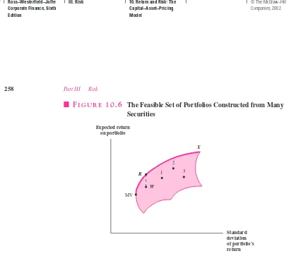
The previous discussion concerned two securities. We found that a simple curve sketched out all the possible portfolios. Because investors generally hold more than two securities, we should look at the same graph when more than two securities are held. The shaded area in Fig-ure 10.6 represents the opportunity set or feasible set when many securities are considered. The shaded area represents all the possible combinations of expected return and standard de-viation for a portfolio. For example, in a universe of 100 securities, point 1 might represent a portfolio of, say, 40 securities. Point 2 might represent a portfolio of 80 securities. Point 3 might represent a different set of 80 securities, or the same 80 securities held in different pro-portions, or something else. Obviously, the combinations are virtually endless. However, note
that all possible combinations fit into a confined region. No security or combination of secu-rities can fall outside of the shaded region. That is, no one can choose a portfolio with an ex-pected return above that given by the shaded region. Furthermore, no one can choose a port-folio with a standard deviation below that given in the shady area. Perhaps more surprisingly, no one can choose an expected return below that given in the curve. In other words, the cap-ital markets actually prevent a self-destructive person from taking on a guaranteed loss.6
So far, Figure 10.6 is different from the earlier graphs. When only two securities are involved, all the combinations lie on a single curve. Conversely, with many securities the combinations cover an entire area. However, notice that an individual will want to be some-where on the upper edge between MV and X.The upper edge, which we indicate in Figure 10.6 by a thick curve, is called the efficient set.Any point below the efficient set would re-ceive less expected return and the same standard deviation as a point on the efficient set. For example, consider Ron the efficient set and Wdirectly below it. If Wcontains the risk you desire, you should choose Rinstead in order to receive a higher expected return.
In the final analysis, Figure 10.6 is quite similar to Figure 10.3. The efficient set in Figure 10.3 runs from MV to Supertech. It contains various combinations of the securities Supertech and Slowpoke. The efficient set in Figure 10.6 runs from MV to X.It contains various combinations of many securities. The fact that a whole shaded area appears in Figure 10.6 but not in Figure 10.3 is just not an important difference; no investor would choose any point below the efficient set in Figure 10.6 anyway.
We mentioned before that an efficient set for two securities can be traced out easily in the real world. The task becomes more difficult when additional securities are included be-cause the number of observations grows. For example, using subjective analysis to estimate expected returns and standard deviations for, say, 100 or 500 securities may very well be-come overwhelming, and the difficulties with correlations may be greater still. There are al-most 5,000 correlations between pairs of securities from a universe of 100 securities.
6
Of course, someone dead set on parting with his money can do so. For example, he can trade frequently without purpose, so that commissions more than offset the positive expected returns on the portfolio.
Expected return on portfolio
Standard deviation of portfolio’s return X
R 1
W
2
3
MV
Though much of the mathematics of efficient-set computation had been derived in the 1950s,7the high cost of computer time restricted application of the principles. In recent years, the cost has been drastically reduced. A number of software packages allow the cal-culation of an efficient set for portfolios of moderate size. By all accounts these packages sell quite briskly, so that our discussion above would appear to be important in practice.
Variance and Standard Deviation in a Portfolio of Many Assets
We earlier calculated the formulas for variance and standard deviation in the two-asset case. Because we considered a portfolio of many assets in Figure 10.6, it is worthwhile to calcu-late the formulas for variance and standard deviation in the many-asset case. The formula for the variance of a portfolio of many assets can be viewed as an extension of the formula for the variance of two assets.
To develop the formula, we employ the same type of matrix that we used in the two-asset case. This matrix is displayed in Table 10.4. Assuming that there are Nassets, we write the numbers 1 through Non the horizontal axis and 1 through Non the vertical axis. This creates a matrix of NN N2boxes. The variance of the portfolio is the sum of the terms in all the boxes.
Consider, for example, the box in the second row and the third column. The term in the box is X2X3Cov(R2,R3). X2and X3are the percentages of the entire portfolio that are in-vested in the second asset and the third asset, respectively. For example, if an individual with a portfolio of $1,000 invests $100 in the second asset,X2 10% ($100/$1,000). Cov(R3,R2) is the covariance between the returns on the third asset and the returns on the second asset. Next, note the box in the third row and the second column. The term in this box is X3X2Cov(R3,R2). Because Cov(R3,R2) Cov(R2,R3), both boxes have the same value. The second security and the third security make up one pair of stocks. In fact, every pair of stocks appears twice in the table, once in the lower left-hand side and once in the upper right-hand side.
7
The classic treatise is Harry Markowitz,Portfolio Selection(New York: John Wiley & Sons, 1959). Markowitz won the Nobel Prize in economics in 1990 for his work on modern portfolio theory.
■
T
A B L E1 0 . 4
Matrix Used to Calculate the Variance of a PortfolioThe variance of the portfolio is the sum of the terms in all the boxes.
!iis the standard deviation of stock i.
Cov(Ri,Rj) is the covariance between stock iand stock j.
Terms involving the standard deviation of a single security appear on the diagonal. Terms involving covariance between two securities appear off the diagonal.
Now consider boxes on the diagonal. For example, the term in the first box on the di-agonal is . Here, is the variance of the return on the first security.
Thus, the diagonal terms in the matrix contain the variances of the different stocks. The off-diagonal terms contain the covariances. Table 10.5 relates the numbers of diagonal and off-diagonal elements to the size of the matrix. The number of diagonal terms (number of variance terms) is always the same as the number of stocks in the portfolio. The number of off-diagonal terms (number of covariance terms) rises much faster than the number of di-agonal terms. For example, a portfolio of 100 stocks has 9,900 covariance terms. Since the variance of a portfolio’s returns is the sum of all the boxes, we have:
The variance of the return on a portfolio with many securities is more dependent on the co-variances between the individual securities than on the co-variances of the individual securities.
• What is the formula for the variance of a portfolio for many assets? • How can the formula be expressed in terms of a box or matrix?
10.6
D
IVERSIFICATION
: A
N
E
XAMPLE
The preceding point can be illustrated by altering the matrix in Table 10.4 slightly. Suppose that we make the following three assumptions:
1. All securities possess the same variance, which we write as . In other words, for every security.
2. All covariances in Table 10.4 are the same. We represent this uniform covariance as . In other words, for every pair of securities. It can easily be shown that
. Function of the Number of Stocks in the Portfolio
Number of Number of Variance Covariance
Terms Terms
Number of Total (number of (number of
Stocks in Number terms terms
Portfolio of Terms on diagonal) off diagonal)
1 1 1 0
In a large portfolio, the number of terms involving covariance between two securities is much greater than the number of terms involving variance of a single security.
3. All securities are equally weighted in the portfolio. Because there are Nassets, the weight of each asset in the portfolio is 1/N.In other words,Xi1/Nfor each security i.
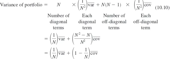
Table 10.6 is the matrix of variances and covariances under these three simplifying assumptions. Note that all of the diagonal terms are identical. Similarly, all of the off-diagonal terms are identical. As with Table 10.4, the variance of the portfolio is the sum of the terms in the boxes in Table 10.6. We know that there are Ndiagonal terms in-volving variance. Similarly, there are N (N!1) off-diagonal terms involving covari-ance. Summing across all the boxes in Table 10.6 we can express the variances of the portfolio as
(10.10)
Number of Each Number of Each
diagonal diagonal off-diagonal off-diagonal
terms term terms term
Equation (10.10) expresses the variance of our special portfolio as a weighted sum of the average security variance and the average covariance.8
1Equation (10.10) is actually a weighted averageof the variance and covariance terms because the weights, 1/N and 1 !1/N, sum to 1.
■
T
A B L E1 0 . 6
Matrix Used to Calculate the Variance of a Portfolio When (a) All Securities Possess the Same Variance, Which We Represent as ; (b) All Pairs of Securities Possess the Same Covariance, Which We Represent as ; (c) All Securities Are Held in the Same Proportion,Now, let’s increase the number of securities in the portfolio without limit. The variance of the portfolio becomes
Variance of portfolio (when N→) (10.11)
This occurs because (1) the weight on the variance term, 1/N,goes to 0 as Ngoes to infin-ity, and (2) the weight on the covariance term, 1 1/N,goes to 1 as Ngoes to infinity.
Formula (10.11) provides an interesting and important result. In our special portfolio, the variances of the individual securities completely vanish as the number of securities be-comes large. However, the covariance terms remain. In fact, the variance of the portfolio becomes the average covariance, . One often hears that one should diversify. In other words, you should not put all your eggs in one basket. The effect of diversification on the risk of a portfolio can be illustrated in this example. The variances of the individual securi-ties are diversified away, but the covariance terms cannot be diversified away.
The fact that part, but not all, of one’s risk can be diversified away should be explored. Consider Mr. Smith, who brings $1,000 to the roulette table at a casino. It would be very risky if he put all his money on one spin of the wheel. For example, imagine that he put the full $1,000 on red at the table. If the wheel showed red, he would get $2,000, but if the wheel showed black, he would lose everything. Suppose, instead, he divided his money over 1,000 different spins by betting $1 at a time on red. Probability theory tells us that he could count on winning about 50 percent of the time. This means that he could count on pretty nearly getting all his original $1,000 back.9In other words, risk is essentially eliminated with 1,000 different spins.
Now, let’s contrast this with our stock market example, which we illustrate in Figure 10.7. The variance of the portfolio with only one security is, of course, because the variance of a portfolio with one security is the variance of the security. The variance of the portfolio drops as more securities are added, which is evidence of the diversification effect. However, unlike Mr. Smith’s roulette example, the portfolio’s variance can never drop to zero. Rather it reaches a floor of , which is the covariance of each pair of securities.10
Because the variance of the portfolio asymptotically approaches , each additional security continues to reduce risk. Thus, if there were neither commissions nor other trans-actions costs, it could be argued that one can never achieve too much diversification. However, there is a cost to diversification in the real world. Commissions per dollar invested fall as one makes larger purchases in a single stock. Unfortunately, one must buy fewer shares of each security when buying more and more different securities. Comparing the costs and benefits of diversification, Meir Statman argues that a portfolio of about 30 stocks is needed to achieve optimal diversification.11
We mentioned earlier that must be greater than . Thus, the variance of a secu-rity’s return can be broken down in the following way:
Total risk of Unsystematic or
individual security Portfolio risk ! diversifiable risk
Total risk,which is in our example, is the risk that one bears by holding onto one secu-rity only. Portfolio riskis the risk that one still bears after achieving full diversification,
var
This example ignores the casino’s cut.
10
Though it is harder to show, this risk reduction effect also applies to the general case where variances and covariances are notequal.
11
which is in our example. Portfolio risk is often called systematicor market riskas well. Diversifiable, unique,or unsystematic riskis that risk that can be diversified away in a large portfolio, which must be by definition.
To an individual who selects a diversified portfolio, the total risk of an individual se-curity is not important. When considering adding a sese-curity to a diversified portfolio, the individual cares about only that portion of the risk of a security that cannot be diversified away. This risk can alternatively be viewed as the contributionof a security to the risk of an entire portfolio. We will talk later about the case where securities make different contri-butions to the risk of the entire portfolio.
Risk and the Sensible Investor
Having gone to all this trouble to show that unsystematic risk disappears in a well-diversified portfolio, how do we know that investors even want such portfolios? Suppose they like risk and don’t want it to disappear?
We must admit that, theoretically at least, this is possible, but we will argue that it does not describe what we think of as the typical investor. Our typical investor is risk averse.
Risk-averse behavior can be defined in many ways, but we prefer the following example: A fair gamble is one with zero expected return; a risk-averse investor would prefer to avoid fair gambles.
Why do investors choose well-diversified portfolios? Our answer is that they are risk averse, and risk-averse people avoid unnecessary risk, such as the unsystematic risk on a stock. If you do not think this is much of an answer, consider whether you would take on such a risk. For example, suppose you had worked all summer and had saved $5,000, which
varcov
cov Variance
of portfolio’s
return
Number of securities Diversifiable risk,
unique risk, or unsystematic risk
Portfolio risk, market risk, or systematic risk var
cov
1 2 3 4
■
F
I G U R E1 0 . 7
Relationship between the Variance of a Portfolio’s Return and the Number of Securities in the Portfolio**This graph assumes
a.All securities have constant variance, var. b.All securities have constant covariance, cov. c.All securities are equally weighted in portfolio.
you intended to use for your college expenses. Now, suppose someone came up to you and offered to flip a coin for the money: heads, you would double your money, and tails, you would lose it all.
Would you take such a bet? Perhaps you would, but most people would not. Leaving aside any moral question that might surround gambling and recognizing that some people would take such a bet, it’s our view that the average investor would not.
To induce the typical risk-averse investor to take a fair gamble, you must sweeten the pot. For example, you might need to raise the odds of winning from 50–50 to 70–30 or higher. The risk-averse investor can be induced to take fair gambles only if they are sweet-ened so that they become unfair to the investor’s advantage.
• What are the two components of the total risk of a security? • Why doesn’t diversification eliminate all risk?
10.7
R
ISKLESS
B
ORROWING AND
L
ENDING
Figure 10.6 assumes that all the securities on the efficient set are risky. Alternatively, an in-vestor could combine a risky investment with an investment in a riskless or risk-free secu-rity, such as an investment in United States Treasury bills. This is illustrated in the follow-ing example.
E
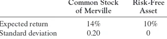
XAMPLEMs. Bagwell is considering investing in the common stock of Merville Enter-prises. In addition, Ms. Bagwell will either borrow or lend at the risk-free rate. The relevant parameters are
Common Stock Risk-Free
of Merville Asset
Expected return 14% 10%
Standard deviation 0.20 0
Suppose Ms. Bagwell chooses to invest a total of $1,000, $350 of which is to be in-vested in Merville Enterprises and $650 placed in the risk-free asset. The expected return on her total investment is simply a weighted average of the two returns:
Expected return on portfolio
composed of one riskless 0.114 (0.35 0.14) !(0.65 0.10) (10.12) and one risky asset
Because the expected return on the portfolio is a weighted average of the expected return on the risky asset (Merville Enterprises) and the risk-free return, the calcu-lation is analogous to the way we treated two risky assets. In other words, equa-tion (10.3) applies here.
Using equation (10.4), the formula for the variance of the portfolio can be written as
X2Merville" 2
Merville !2XMervilleXRisk-free"Merville, Risk-free!X 2 Risk-free"
2 Risk-free
QUESTIONS
C
O
N
CE
P
T
However, by definition, the risk-free asset has no variability. Thus, both
Merville, Risk-freeand are equal to zero, reducing the above expression to
Variance of portfolio composed
of one riskless and one risky asset (10.13)
The standard deviation of the portfolio is
Standard deviation of portfolio composed
of one riskless and one risky asset (10.14)
XMervilleMerville 0.35 !0.20 0.07
The relationship between risk and expected return for one risky and one risk-less asset can be seen in Figure 10.8. Ms. Bagwell’s split of 35–65 percent between the two assets is represented on a straightline between the risk-free rate and a pure investment in Merville Enterprises. Note that, unlike the case of two risky assets, the opportunity set is straight, not curved.
Suppose that, alternatively, Ms. Bagwell borrows $200 at the risk-free rate. Combining this with her original sum of $1,000, she invests a total of $1,200 in Merville. Her expected return would be
Expected return on portfolio
formed by borrowing 14.8% 1.20 !0.14 "(#0.2 !0.10) to invest in risky asset
Here, she invests 120 percent of her original investment of $1,000 by borrowing 20 percent of her original investment. Note that the return of 14.8 percent is greater than the 14-percent expected return on Merville Enterprises. This occurs because she is borrowing at 10 percent to invest in a security with an expected return greater than 10 percent.
X2
Merville2Merville 0.352! 0.202 0.0049
Risk-free2
Expected return on portfolio (%)
Standard deviation of portfolio’s return (%)
120% in Merville Enterprises –20% in risk-free assets (borrowing at risk-free rate)
Borrowing to invest in Merville when the borrowing rate is greater than the lending rate Merville Enterprises
35% in Merville Enterprises 65% in risk-free assets
20 14
10=RF
The standard deviation is
Standard deviation of portfolio formed
by borrowing to invest in risky asset 0.24 1.20 0.2
The standard deviation of 0.24 is greater than 0.20, the standard deviation of the Merville investment, because borrowing increases the variability of the invest-ment. This investment also appears in Figure 10.8.
So far, we have assumed that Ms. Bagwell is able to borrow at the same rate at which she can lend.12Now let us consider the case where the borrowing rate is above the lending rate. The dotted line in Figure 10.8 illustrates the opportunity set for borrowing opportunities in this case. The dotted line is below the solid line because a higher borrowing rate lowers the expected return on the investment.
The Optimal Portfolio
The previous section concerned a portfolio formed between one riskless asset and one risky asset. In reality, an investor is likely to combine an investment in the riskless asset with a portfolioof risky assets. This is illustrated in Figure 10.9.
Consider point Q,representing a portfolio of securities. Point Qis in the interior of the feasible set of risky securities. Let us assume the point represents a portfolio of 30 percent in AT&T, 45 percent in General Motors (GM), and 25 percent in IBM. Individuals
com-12
Surprisingly, this appears to be a decent approximation because a large number of investors are able to borrow from a stockbroker (called going on margin) when purchasing stocks. The borrowing rate here is very near the riskless rate of interest, particularly for large investors. More will be said about this in a later chapter.
Risk-free
■
F
I G U R E1 0 . 9
Relationship between Expected Return and Standard Deviation for an Investment in a Combination of Risky Securities and the Riskless Assetbining investments in Qwith investments in the riskless asset would achieve points along the straight line from RFto Q.We refer to this as line I.For example, point 1on the line rep-resents a portfolio of 70 percent in the riskless asset and 30 percent in stocks represented by Q.An investor with $100 choosing point 1as his portfolio would put $70 in the risk-free asset and $30 in Q.This can be restated as $70 in the riskless asset, $9 (0.3 $30) in AT&T,
$13.50 (0.45 $30) in GM, and $7.50 (0.25 $30) in IBM. Point 2also represents a
port-folio of the risk-free asset and Q,with more (65%) being invested in Q.
Point 3is obtained by borrowing to invest in Q.For example, an investor with $100 of his own would borrow $40 from the bank or broker in order to invest $140 in Q.This can be stated as borrowing $40 and contributing $100 of one’s money in order to invest $42 (0.3 $140) in
AT&T, $63 (0.45 $140) in GM, and $35 (0.25 $140) in IBM. The above investments can be summarized as:
Point 1 Point 3
Point Q (lending $70) (borrowing $40)
AT&T $ 30 $ 9 $ 42
GM 45 13.50 63
IBM 25 7.50 35
Risk-free ____0 _______70.00 ____40
Total investment $100 $100 $100
Though any investor can obtain any point on line I,no point on the line is optimal. To see this, consider line II,a line running from RFthrough A.Point Arepresents a portfolio of risky securities. Line IIrepresents portfolios formed by combinations of the risk-free as-set and the securities in A.Points between RFand Aare portfolios in which some money is invested in the riskless asset and the rest is placed in A.Points past Aare achieved by bor-rowing at the riskless rate to buy more of Athan one could with one’s original funds alone. As drawn, line IIis tangent to the efficient set of risky securities. Whatever point an in-dividual can obtain on line I,he can obtain a point with the same standard deviation and a higher expected return on line II.In fact, because line IIis tangent to the efficient set of risky assets, it provides the investor with the best possible opportunities. In other words, line IIcan be viewed as the efficient set of allassets, both risky and riskless. An investor with a fair de-gree of risk aversion might choose a point between RFand A,perhaps point 4.An individual with less risk aversion might choose a point closer to Aor even beyond A.For example, point 5corresponds to an individual borrowing money to increase his investment in A.
The graph illustrates an important point. With riskless borrowing and lending, the port-folio of riskyassets held by any investor would always be point A.Regardless of the in-vestor’s tolerance for risk, he would never choose any other point on the efficient set of risky assets (represented by curve XAY) nor any point in the interior of the feasible region. Rather, he would combine the securities of Awith the riskless assets if he had high aversion to risk. He would borrow the riskless asset to invest more funds in Ahad he low aversion to risk.
This result establishes what financial economists call the separation principle.That is, the investor’s investment decision consists of two separate steps:
2. The investor must now determine how he will combine point A,his portfolio of risky assets, with the riskless asset. He might invest some of his funds in the riskless asset and some in portfolio A.He would end up at a point on the line between RFand Ain this case. Alternatively, he might borrow at the risk-free rate and contribute some of his own funds as well, investing the sum in portfolio A.He would end up at a point on line II be-yond A.His position in the riskless asset, that is, his choice of where on the line he wants to be, is determined by his internal characteristics, such as his ability to tolerate risk.
• What is the formula for the standard deviation of a portfolio composed of one riskless and one risky asset?
• How does one determine the optimal portfolio among the efficient set of risky assets?
10.8
M
ARKET
E
QUILIBRIUM
Definition of the Market-Equilibrium Portfolio
The above analysis concerns one investor. His estimates of the expected returns and vari-ances for individual securities and the covarivari-ances between pairs of securities are his and his alone. Other investors would obviously have different estimates of the above variables. How-ever, the estimates might not vary much because all investors would be forming expectations from the same data on past price movements and other publicly available information.
Financial economists often imagine a world where all investors possess the sameestimates on expected returns, variances, and covariances. Though this can never be literally true, it can be thought of as a useful simplifying assumption in a world where investors have access to sim-ilar sources of information. This assumption is called homogeneous expectations.13
If all investors had homogeneous expectations, Figure 10.9 would be the same for all individuals. That is, all investors would sketch out the same efficient set of risky assets be-cause they would be working with the same inputs. This efficient set of risky assets is rep-resented by the curve XAY.Because the same risk-free rate would apply to everyone, all in-vestors would view point Aas the portfolio of risky assets to be held.
This point Atakes on great importance because all investors would purchase the risky securities that it represents. Those investors with a high degree of risk aversion might com-bine Awith an investment in the riskless asset, achieving point 4,for example. Others with low aversion to risk might borrow to achieve, say, point 5.Because this is a very important conclusion, we restate it:
In a world with homogeneous expectations, all investors would hold the portfolio of risky assets represented by point A.
If all investors choose the same portfolio of risky assets, it is possible to determine what that portfolio is. Common sense tells us that it is a market-value-weighted portfolio of all existing securities. It is the market portfolio.
In practice, financial economists use a broad-based index such as the Standard & Poor’s (S&P) 500 as a proxy for the market portfolio. Of course all investors do not hold the same portfolio in practice. However, we know that a large number of investors hold
di-13
The assumption of homogeneous expectations states that all investors have the same beliefs concerning returns, variances, and covariances. It does not say that all investors have the same aversion to risk.
QUESTIONS
C
O
N
CE
P
T