The Design and Analysis of Parallel Algorithms

(1)

The Design and Analysis

of

Parallel Algorithms

Selim

G .

Akl

Queen's nioersity Kingston, Ontario, Canada

(2)

A k l . G.

T h e d e s i g n a n d o f p a r a l l e l a l g o r i t h m s by G. A k l . p. cm.

B i b l i o g r a p h y : p. I n c l u d e s I n d e x . I S B N 0-13-200056-3

1 . P a r a l l e l p r o g r a m m i n g ( C o m p u t e r s c i e n c e ) 2 . A l g o r i t h m s . I . T i t l e .

1989

19 C I P

supervision, Ann Mohan

Cover design: Lundgren Graphics Ltd. Manufacturing buyer: Mary

1989 by Prentice-Hall, Inc. A Division of Simon Schuster Englewood Cliffs, New Jersey 07632

Printed in the United States of America 1 0 9 8 7 6 5 4 3 2 1

ISBN

Prentice-Hall International (UK) Limited, London

Prentice-Hall of Australia Pty. Limited, Sydney

Prentice-Hall Canada Inc., Toronto

Prentice-Hall Hispanoamericana, S.A., Mexico

Prentice-Hall of India Private Limited, New Delhi Prentice-Hall of Japan, Inc., Tokyo

Simon Schuster Asia Pte. Ltd., Singapore

(3)

To Theo,

(4)

6

GENERATING PERMUTATIONS AND COMBINATIONS 141

6.1 Introduction, 141

6.2 Sequential Algorithms, 142

6.2.1 Generating Permutations Lexicographically, 143

6.2.2 Numbering Permutations, 145

6.2.3 Generating Combinations Lexicographically, 147

6.2.4 Numbering Combinations, 148

6.3 Generating Permutations I n Parallel, 150

6.3.1 Adapting a Sequential Algorithm, 150

6.3.2 An Adaptive Permutation Generator, 156

6.3.3 Parallel Permutation Generator for Few Processors, 157

6.4 Generating Combinations In Parallel, 158

6.4.1 A Fast Combination Generator, 158

6.4.2 An Adaptive Combination Generator, 162

6.5 Problems, 163

(7)

viii

7.4.1 Linear Array Multiplication, 188 7.4.2 Tree Multiplication, 190

8.2 Solving Systems of Linear Equations, 201 8.2.1 An SIMD Algorithm, 201

8.2.2 An MIMD Algorithm, 203

8.3 Finding Roots of Nonlinear Equations, 206 8.3.1 An SIMD Algorithm, 206

8.3.2 An MIMD Algorithm, 209

8.4 Solving Partial Differential Equations, 21 2 8.5 Computing Eigenvalues, 21 5

8.6 Problems, 221

COMPUTING FOURIER TRANSFORMS 231

9.1.1 The Fast Fourier Transform, 231 9.1.2 An Application of the FFT, 232 9.1.3 Computing the DFT In Parallel, 233 9.2 Direct Computation of the DFT, 233

9.2.1 Computing the Matrix 234

9.2.2 Computing the DFT, 235

9.3 A Parallel FFT Algorithm, 238 9.4 Problems, 242

(8)

GRAPHTHEORY 251

10.1 Introduction, 251 10.2 Definitions, 251

10.3 Computing the Connectivity Matrix, 254 10.4 Finding Connected Components, 256 10.5 All-Pairs Shortest Paths, 257

10.6 Computing the Minimum Spanning Tree, 261 10.7 Problems, 266

10.8 Bibliographical Remarks, 271 10.9 References, 272

COMPUTATIONAL GEOMETRY 278

1 1 Introduction, 278

11.2 An Inclusion Problem, 279 11.2.1 Point in Polygon, 280

11.2.2 Point in Planar Subdivision, 283 11.3 An Intersection Problem, 285 11.4 A Proximity Problem, 287 11.5 A Construction Problem, 288

11.5.1 Lower Bound, 289

12.2 Sequential Tree Traversal, 31 2 12.3 Basic Design Principles, 31 7

12.3.1 The Minimal Alpha-Beta Tree, 318 12.3.2 Model of Computation, 319 12.3.3 Objectives and Methods, 320 12.4 The Algorithm, 323

12.4.1 Procedures and Processes, 323 12.4.2 Semaphores, 323

12.4.3 Score Tables, 324 12.5 Analysis and Examples, 327

12.5.1 Parallel Cutoffs, 327 12.5.2 Storage Requirements, 33 1 12.6 Problems, 336

(9)

Contents

DECISION A N D OPTIMIZATION 341

13.2 Computing Prefix Sums, 341

13.2.1 A Specialized Network, 342

13.2.2 Using the Connection, 343 13.2.3 Prefix Sums on a Tree, 346

13.2.4 Prefix Sums on a Mesh, 349

13.3 Applications, 351

13.3.1 Job Sequencing with Deadlines, 35 1 13.3.2 The Knapsack Problem, 352 13.3.3 Mesh Solutions, 354

13.4 Problems, 355

THE BIT COMPLEXITY OF PARALLEL COMPUTATIONS 361

14.2 Adding Two Integers, 363 14.3 Adding n Integers, 364

14.3.1 Addition Tree, 364 14.3.2 Addition Mesh, 366

14.4 Multiplying Two Integers, 366

14.4.1 Multiplication Tree, 368 14.4.2 Multiplication Mesh, 369

14.5 Computing Prefix Sums, 373

14.5.1 Variable Fan-out, 373 14.5.2 Constant Fan-out, 374

14.6 Matrix Multiplication, 374 14.7 Selection, 376

14.8 Sorting, 381 14.9 Problems, 382

14.1 0 Bibliographical Remarks, 384 1 References, 386

AUTHOR INDEX 389

(10)

Preface

The need for ever faster computers has not ceased since the beginning of the computer era. Every new application seems to push existing computers to their limit. So far, computer manufacturers have kept up with the demand admirably well. In 1948, the electronic components used to build computers could switch from one state to another about 10,000 times every second. The switching time of this year's components is approximately of a second. These figures mean that the number of operations a computer can d o in one second has doubled, roughly every two years, over the past forty years. This is very impressive, but how long can it last? It is generally believed that the trend will remain until the end of this century. It may even be possible to maintain it a little longer by using optically based or even biologically based components. What happens after that?

If the current and contemplated applications of computers are any indication, our requirements in terms of computing speed will continue, at least at the same rate as in the past, well beyond the year 2000. Already, computers faster than any available today are needed to perform the enormous number of calculations involved in developing cures to mysterious diseases. They are essential to applications where the human ability to recognize complex visual and auditory patterns is to be simulated in real time. And they are indispensable if we are to realize many of humanity's dreams, ranging from reliable long-term weather forecasting to interplanetary travel and outer space exploration. It appears now that parallel processing is the way to achieve these desired computing speeds.

The overwhelming majority of computers in existence today, from the simplest to the most powerful, are conceptually very similar to one another. Their architecture and mode of operation follow, more or less, the same basic design principles formulated in the late 1940s and attributed to John von Neumann. The ingenious scenario is very simple and essentially goes as follows: A control unit fetches an instruction and its operands from a memory unit and sends them to a processing unit; there the instruction is executed and the result sent back to memory. This sequence of events is repeated for each instruction. There is only one unit of each kind, and only

(11)

xii Preface

With parallel processing the situation is entirely different. A parallel computer is one that consists of a collection of processing units, or processors, that cooperate to solve a problem by working simultaneously on different parts of that problem. The number of processors used can range from a few tens to several millions. As a result, the time required to solve the problem by a traditional uniprocessor computer is significantly reduced. This approach is attractive for a number of reasons. First, for many computational problems, the natural solution is a parallel one. Second, the cost and size of computer components have declined so sharply in recent years that parallel computers with a large number of processors have become feasible. And, third, it is possible in parallel processing to select the parallel architecture that is best suited to solve the problem or class of problems under consideration. Indeed, architects of parallel computers have the freedom to decide how many processors are to be used, how powerful these should be, what interconnection network links them to one another, whether they share a common memory, to what extent their operations are to be carried out synchronously, and a host of other issues. This wide range of choices has been reflected by the many theoretical models of parallel computation proposed as well as by the several parallel computers that were actually built.

Parallelism is sure to change the way we think about and use computers. It promises to put within our reach solutions to problems and frontiers of knowledge never dreamed of before. The rich variety of architectures will lead to the discovery of novel and more efficient solutions to both old and new problems. It is important therefore to ask: How d o we solve problems on a parallel computer? The primary ingredient in solving a computational problem on any computer is the solution method, or algorithm. This book is about algorithms for parallel computers. It describes how to go about designing algorithms that exploit both the parallelism inherent in the problem and that available on the computer. It also shows how to analyze these algorithms in order to evaluate their speed and cost.

The computational problems studied in this book are grouped into three classes: (1) sorting, searching, and related problems; (2) combinatorial and numerical problems; and (3) problems arising in a number of application problems were chosen due to their fundamental nature. It is shown how a parallel algorithm is designed and analyzed to solve each problem. In some cases, several algorithms are presented that perform the same job, each on a different model of parallel computation. Examples are used as often as possible to illustrate the algorithms. Where necessary, a sequential algorithm is outlined for the problem at hand. Additional algorithms are briefly described in the Problems and Bibliographical Remarks sections. A list of references to other publications, where related problems and algorithms are treated, is provided at the end of each chapter.

(12)

models of computation and the design and analysis of parallel algorithms. It is assumed that the reader possesses the background normally provided by an undergraduate introductory course on the design and analysis of algorithms.

The most pleasant part of writing a book is when one finally gets a chance to thank those who helped make the task an enjoyable one. Four people deserve special credit: Ms. Irene prepared the electronic version of the manuscript with her natural cheerfulness and unmistakable talent. The diagrams are the result of Mr. Mark Attisha's expertise, enthusiasm, and skill. Dr. Bruce Chalmers offered numerous trenchant and insightful comments on an early draft. Advice and assistance on matters big and small were provided generously by Mr. Thomas Bradshaw. I also wish to acknowledge the several helpful suggestions made by the students in my CISC-867 class at Queen's. The support provided by the staff of Prentice Hall at every stage is greatly appreciated

Finally, I am indebted to my wife, Karolina, and to my two children, Sophia and Theo, who participated in this project in more ways than I can mention. Theo, in particular, spent the first year of his life examining, from a vantage point, each word as it appeared on my writing pad.

(13)

Introduction

1.1 THE NEED FOR PARALLEL COMPUTERS

A battery of satellites in outer space are collecting data at the rate of bits per second. The data represent information on the earth's weather, pollution, agriculture, and natural resources. In order for this information to be used in a timely fashion, it needs to be processed at a speed of at least operations per second.

Back on earth, a team of surgeons wish to view on a special display a reconstructed three-dimensional image of a patient's body in preparation for surgery. They need to be able to rotate the image at will, obtain a cross-sectional view of an organ, observe it in living detail, and then perform a simulated surgery while watching its effect, all without touching the patient. A minimum processing speed of operations per second would make this approach worthwhile.

The preceding two examples are representative of applications where trem- endously fast computers are needed to process vast amounts of data or to perform a large number of calculations quickly (or at least within a reasonable length of time). Other such applications include aircraft testing, the development of new drugs, oil exploration, modeling fusion reactors, economic planning, cryptanalysis, managing large databases, astronomy, biomedical analysis, real-time speech recognition, robo- tics, and the solution of large systems of partial differential equations arising from numerical simulations in disciplines as diverse as seismology, aerodynamics, and atomic, nuclear, and plasma physics. No computer exists today that can deliver the processing speeds required by these applications. Even the so-called supercomputers

peak at a few billion operations per second.

Over the past forty years dramatic increases in computing speed were achieved. Most of these were largely due to the use of inherently faster electronic components by computer manufacturers. As we went from relays to vacuum tubes to transistors and from to medium to large and then to very large scale integration, we

often in amazement-the growth in size and range of the computational problems that we could solve.

(14)

approximately equal to 3 x meters per second. Now, assume that an electronic device can perform operations per second. Then it takes longer for a signal to travel between two such devices one-half of a millimeter apart than it takes for either of them to process it. In other words, all the gains in speed obtained by building superfast electronic components are lost while one component is waiting to receive some input from another one. Why then (one is compelled to ask) not put the two communicating components even closer together? Again, physics tells us that the reduction of distance between electronic devices reaches a point beyond which they begin to interact, thus reducing not only their speed but also their reliability.

It appears that the only way around this problem is to use parallelism. The idea here is that if several operations are performed simultaneously, then the time taken by a computation can be significantly reduced. This is a fairly intuitive notion, and one to which we are accustomed in any organized society. We know that several people of comparable skills can usually finish a job in a fraction of the time taken by one individual. From mail distribution to harvesting and from office to factory work, our everyday life offers numerous examples of parallelism through task sharing.

Even in the field of computing, the idea of parallelism is not entirely new and has taken many forms. Since the early days of information processing, people realized that it is greatly advantageous to have the various components of a computer do different things at the same time. Typically, while the central processing unit is doing calculations, input can be read from a magnetic tape and output produced on a line printer. In more advanced machines, there are several simple processors each specializing in a given computational task, such as operations on floating-point numbers, for example. Some of today's most powerful computers contain two or more processing units that share among themselves the jobs submitted for processing.

In each of the examples just mentioned, parallelism is exploited profitably, but nowhere near its promised power. Strictly speaking, none of the machines discussed is truly a parallel computer. In the modern paradigm that we are about to describe, however, the idea of parallel computing can realize its full potential. Here, our computational tool is a parallel computer, that is, a computer with many processing units, or processors. Given a problem to be solved, it is broken into a number of subproblems. All of these subproblems are now solved simultaneously, each on a different processor. The results are then combined to produce an answer to the original problem. This is a radical departure from the model of computation adopted for the past forty years in building computers-namely, the sequential uniprocessor machine.

(15)

1.2 Models of Computation 3

With the availability of the hardware, the most pressing question in parallel computing today is: How to program parallel computers to solve problems efficiently and in a practical and economically feasible way? As is the case in the sequential world, parallel computing requires algorithms, programming languages and com- pilers, as well as operating systems in order to actually perform a computation on the parallel hardware. All these ingredients of parallel computing are currently receiving a good deal of well-deserved attention from researchers.

This book is about one (and perhaps the most fundamental) aspect of parallelism, namely, parallel algorithms. A parallel algorithm is a solution method for a given problem destined to be performed on a parallel computer. In order to properly design such algorithms, one needs to have a clear understanding of the model of computation underlying the parallel computer.

1.2 MODELS OF COMPUTATION

Any computer, whether sequential or parallel, operates by executing instructions on data. A stream of instructions (the algorithm) tells the computer what to do at each step. A stream of data (the input to the algorithm) is affected by these instructions. Depending on whether there is one or several of these streams, we can distinguish among four classes of computers:

1. Single Instruction stream, Single Data stream (SISD) 2. Multiple Instruction stream, Single Data stream (MISD)

3. Single Instruction stream, Multiple Data stream (SIMD) 4. Multiple Instruction stream, Multiple Data stream (MIMD).

We now examine each of these classes in some detail. In the discussion that follows we shall not be concerned with input, output, or peripheral units that are available on every computer.

1.2.1 Computers

A computer in this class consists of a single processing unit receiving a single stream of instructions that operate on a single stream of data, as shown in Fig. 1.1. At each step during the computation the control unit emits one instruction that operates on a datum obtained from the memory unit. Such an instruction may tell the processor, for

Figure 1.1 SISD computer.

MEMORY

STREAM

PROCESSOR, CONTROL

(16)

example, to perform some arithmetic or logic operation on the datum and then put it back in memory.

The overwhelming majority of computers today adhere to this model invented by John von Neumann and his collaborators in the late 1940s. An algorithm for a computer in this class is said to be sequential (or serial).

Example 1.1

In order to compute the sum of n numbers, the processor needs to gain access to the memory n consecutive times and each time receive one number. There are also n 1 additions involved that are executed in sequence. Therefore, this computation requires on the order of n operations in total.

This example shows that algorithms for SISD computers do not contain any parallelism. The reason is obvious, there is only one processor! In order to obtain from a computer the kind of parallel operation defined earlier, it will need to have several processors. This is provided by the next three classes of computers, the classes of interest in this book. In each of these classes, a computer possesses N processors, where N 1.

1.2.2 Computers

Here, N processors each with its own control unit share a common memory unit where data reside, as shown in Fig. There are N streams of instructions and one stream of data. At each step, one datum received from memory is operated upon by all the processors simultaneously, each according to the instruction it receives from its control. Thus, parallelism is achieved by letting the processors do different things at the same time on the same datum. This class of computers lends itself naturally to those computations requiring an input to be subjected to several operations, each receiving the input in its original form. Two such computations are now illustrated.

(17)

1.2 Models of Computation

Example 1.2

It is required to determine whether a given positive integer z has no divisors except 1 and itself. The obvious solution to this problem is to try all possible divisors of z: If none of these succeeds in dividing z, then z is said to be prime; otherwise z is said to be composite. We can implement this solution as a parallel algorithm on an MISD computer. The idea is to split the job of testing potential divisors among processors. Assume that there are as many processors on the parallel computer as there are potential divisors of z. All processors take z as input, then each tries to divide it by its associated potential divisor and issues an appropriate output based on the result. Thus it is possible to determine in one step whether z is prime. More realistically, if there are fewer processors than potential divisors, then each processor can be given the job of testing a different subset of these divisors. In either case, a substantial speedup is obtained over a purely sequential implementation.

Although more efficient solutions to the problem of testing exist, we have chosen the simple one as it illustrates the point without the need for much mathematical sophistication.

Example 1.3

In many applications, we often need to determine to which of a number of classes does a given object belong. The object may be a mathematical one, where it is required to associate a number with one of several sets, each with its own properties. Or it may be a physical one: A robot scanning the deep-sea bed "sees" different objects that it has to recognize in order to distinguish among fish, rocks, algae, and so on. Typically, membership of the object is determined by subjecting it to a number of different tests.

The classification process can be done very quickly on an MISD computer with as many processors as there are classes. Each processor is associated with a class and can recognize members of that class through a computational test. Given an object to be classified, it is sent simultaneously to all processors where it is tested in parallel. The object belongs to the class associated with that processor that reports the success of its test. (Of course, it may be that the object does not belong to any of the classes tested for, in which case all processors report failure.) As in example 1.2, when fewer processors than classes are available, several tests are performed by each processor; here, however, in reporting success, a processor must also provide the class to which the object belongs.

The preceding examples show that the class of MISD computers could be extremely useful in many applications. It is also apparent that the kind of computations that can be carried out efficiently o n these computers are of a rather specialized nature. For most applications, MISD computers would be rather awkward t o use. Parallel computers that are more flexible, and hence suitable for a wide range of problems, are described in the next two sections.

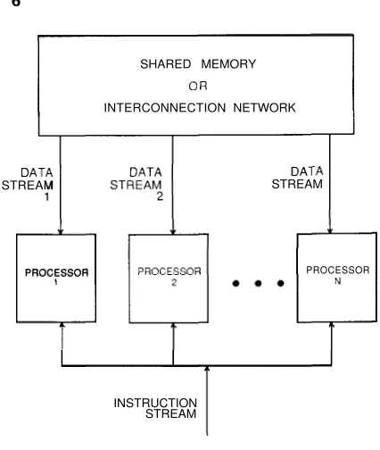
1.2.3 D Computers

I n this class, a parallel computer consists of N identical processors, as shown in Fig. 1.3.

(18)

STREAM

PROCESSOR

SHARED MEMORY

INTERCONNECTION NETWORK

STREAM

PROCESSOR

INSTRUCTION STREAM

CONTROL

Figure 1.3 SIMD computer.

programs and data. All processors operate under the control of a single instruction stream issued by a central control unit. Equivalently, the N processors may be assumed to hold identical copies of a single program, each processor's copy being stored in its local memory. There are N data streams, one per processor.

The processors operate synchronously: At each step, all processors execute the same instruction, each on a different datum. The instruction could be a simple one (such as adding or comparing two numbers) or a complex one (such as merging two lists of numbers). Similarly, the datum may be simple (one number) or complex (several numbers). Sometimes, it may be necessary to have only a subset of the processors execute an instruction. This information can be encoded in the instruction itself, thereby telling a processor whether it should be active (and execute the instruction) or

inactive (and wait for the next instruction). There is a mechanism, such as a global clock, that ensures lock-step operation. Thus processors that are inactive during an instruction or those that complete execution of the instruction before others may stay idle until the next instruction is issued. The time interval between two instructions may be fixed or may depend on the instruction being executed.

(19)

1.2.3.1 Shared-Memory ( S M ) SIMD Computers. This class is also known in the literature as the Parallel Random-Access Machine (PRAM) model. Here, the N processors share a common memory that they use in the same way a group of people may use a bulletin board. When two processors wish to communicate, they do so through the shared memory. Say processor i wishes to pass a number to processor j. This is done in two steps. First, processor i writes the number in the shared memory at a given location known to processor j. Then, processor j reads the number from that location.

During the execution of a parallel algorithm, the N processors gain access to the shared memory for reading input data, for reading or writing intermediate results, and for writing final results. The basic model allows all processors to gain access to the shared memory simultaneously if the memory locations they are trying to read from or write into are different. However, the class of shared-memory SIMD computers can be further divided into four subclasses, according to whether two or more processors can gain access to the same memory location simultaneously:

(i) Exclusive-Read, Exclusive-Write (EREW) SM SIMD Computers. Access

to memory locations is exclusive. In other words, no two processors are allowed simultaneously to read from or write into the same memory location.

(ii) Concurrent-Read, Exclusive-Write (CREW) SM SIMD Computers.

Multiple processors are allowed to read from the same memory location but the right to write is still exclusive: No two processors are allowed to write into the same location simultaneously.

Exclusive-Read, Concurrent-Write (ERCW) SM SIMD Computers.

Multiple processors are allowed to write into the same memory location but read accesses remain exclusive.

(iv) Concurrent-Read, Concurrent-Write (CRCW) SM SIMD Computers.

Both multiple-read and multiple-write privileges are granted.

Allowing multiple-read accesses to the same address in memory should in principle pose no problems (except perhaps some technological ones to be discussed later). Conceptually, each of the several processors reading from that location makes a copy of the location's contents and stores it in its own local memory.

With multiple-write accesses, however, difficulties arise. If several processors are attempting simultaneously to store (potentially different) data at a given address, which of them should succeed? In other words, there should be a deterministic way of specifying the contents of that address after the write operation. Several policies have been proposed to resolve such write thus further subdividing classes and (iv). Some of these policies are

(a) the smallest-numbered processor is allowed to write, and access is denied to all other processors;

(b) all processors are allowed to write provided that the quantities they are attempting to store are equal, otherwise access is denied to all processors; and

(20)

A typical representative of t h e class of problems t h a t c a n b e solved o n parallel c o m p u t e r s of t h e SM SIMD family is given i n t h e following example.

Example 1.4

Consider a very large computer file consisting of distinct entries. We shall assume for simplicity that the file is not sorted in any order. (In fact, it may be the case that keeping the file sorted a t all times is impossible or simply inefficient.) Now suppose that it is d o a little better: If the file entries are distributed uniformly over a given range, then half as many steps are required to retrieve

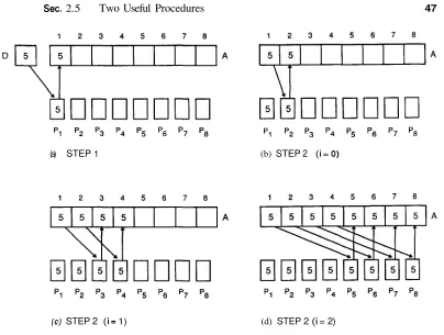
The job can be done a lot faster on an EREW SM SIMD computer with N receive doubles at each stage, broadcasting x to all N processors requires log N

A formal statement of the broadcasting process is given in section

Now the file t o be searched for x is subdivided into that are searched simultaneously by the processors: searches the first elements, searches the second elements, and so on. Since all are of the same size, steps are needed in the worst case t o answer the query about x. In total, therefore, this parallel algorithm requires log N

+

steps in the worst case. O n the average, we can d o better than that (as was done with the SISD computer): A location F holding a Boolean value can be set aside in the shared memory to signal that one of the processors has found the item searched for and, consequently, that all other processors should terminate their search. Initially, F is set t o When a processor finds x in its it sets F to true. At every step of the search all processors check F to see if it is true and stop if this is the case. Unfortunately, this modification of the algorithm does not come for free: log N steps are needed t o broadcast the value of F each time the processors need it. This leads t o a total of log N

+

N steps in the worst case. It is possible to improve this behavior by having the processors either check the value of F a t every (log step, or broadcast it (once true) concurrently with the search process.

'Note that the indexing schemes used for processors in this chapter are for illustration only. Thus, for example, in subsequent chapters a set of N processors may be numbered to N, or to N - 1, whichever is more convenient.

(21)

In order to truly exploit this early termination trick without increasing the worst- case running time, we need to use a more powerful model, namely, a CREW SM SIMD computer. Since concurrent-read operations are allowed, it takes one step for all processors to obtain initially and one step for them to read F each time it is needed. This leads to a worst case of steps.

Finally we note that an even more powerful model is needed if we remove the assumption made at the outset of this example that all entries in the file are distinct. Typically, the file may represent a textual database with hundreds of thousands of articles, each containing several thousand words; It may be necessary to search such a file for a given word x. In this case, more than one entry may be equal to x, and hence more than one processor may need to report success at the same time. This means that two or more processors will attempt to write into location F simultaneously, a situation that can only be handled by a CRCW SM SIMD computer.

Simulating Multiple Accesses on an EREW Computer. The EREW

SM SIMD model of a parallel computer is unquestionably the weakest of the four subclasses of the shared-memory approach, as it restricts its access to a given address to one processor at a time. An algorithm for such a computer must be specifically designed to exclude any attempt by more than one processor to read from o r write into the same location simultaneously. The model is sufficiently flexible, however, to allow the simulation of multiple accesses at the cost of either increasing the space and/or the time requirements of a n algorithm.

Such a simulation may be desirable for one of two reasons:

1. The parallel computer available belongs to the EREW class and thus the only way to execute a CREW, ERCW, or CRCW algorithm is through simulation or 2. parallel computers of the CREW, ERCW, and CRCW models with a very large number of processors are technologically impossible to build at all. Indeed, the number of processors that can be simultaneously connected to a memory location is limited

(i) not only by the physical size of the device used for that location,

(ii) but also by the device's physical properties (such as voltage).

Therefore concurrent access t o memory by an arbitrary number of processors may not be realizable in practice. Again in this case simulation is the only resort to implement an algorithm developed in theory to include multiple accesses.

(i)

N Multiple Accesses. Suppose that we want to run a parallel algorithm involving multiple accesses on an EREW SM SIMD computer with N processors P,,

.

, Suppose further that every multiple access means that all N processors are attempting to read from or write into the same memory location A. We can simulate multiple-read operations on an EREW computer using a broadcast procedure as explained in example 1.4. This way, A can be distributed to all processors in log N steps. Similarly, a procedure symmetrical to broadcasting can be used to handle multiple-write operations. Assume that the N processors are allowed to write in A

simultaneously only if they are all attempting to store the same value. Let the value that is attempting to write be denoted by a,, 1 i N. The procedure to store in A

(22)

1. For 1 i if and are equal, then sets a secondary variable to

The preceding discussion indicates that multiple-read and multiple-write operations by all processors can be simulated on the EREW model. If every step of an algorithm involves multiple accesses of this sort, then in the worst case such a simulation increases the number of steps the algorithm requires by a factor of log N.

(ii) m out of N Multiple Accesses. We now turn to the more general case

where a multiple read from or a multiple write into a memory location does not necessarily implicate all processors. In a typical algorithm, arbitrary subsets of processors may be each attempting to gain access to different locations, one location per subset. Clearly the procedures for broadcasting and storing described in (i) no longer work in this case. Another approach is needed in order to simulate such an algorithm on the EREW model with N processors. Say that the algorithm requires a total of M locations of shared memory. The idea here is to associate with each of the M locations another 2N - 2 locations. Each of the M locations is thought of as the root of a binary tree with N leaves (the tree has depth log N and a total of 2N - 1 nodes). The leaves of each tree are numbered 1 through N and each is associated with the processor with the same number.

When m processors, m N, need to gain access to location A, they can put their requests at the leaves of the tree rooted at A. For a multiple read from location A, the requests trickle (along with the processors) up the tree until one processor reaches the root and reads from A. The value of A is then sent down the tree to all the processors that need it. Similarly, for a multiple-write operation, the processors "carry" the requests up the tree in the manner described in (i) for the store procedure. After log N steps one processor reaches the root and makes a decision about writing. Going up and down the tree of memory locations requires 2 log N steps. The formal description of these simulations, known as multiple broadcasting and multiple storing, respectively, is the subject of section 3.4 and problem 3.33.

Therefore, the price paid for running a parallel algorithm with arbitrary multiple accesses is a (2N - 2)-fold increase in memory requirements. Furthermore, the number of steps is augmented by a factor on the order of log N in the worst case.

Feasibility o f the Shared-Memory Model. _{The SM SIMD computer}

(23)

circuitry is needed to create a path from that processor to the location in memory holding that datum. The cost of such circuitry is usually expressed as the number of logical gates required to decode the address provided by the processor. If the memory consists of M locations, then the cost of the decoding circuitry may be expressed as

f (M) for some cost function If N processors share that memory as in the SM SIMD model, then the cost of the decoding circuitry climbs to N x f (M). For large N and M this may lead to prohibitively large and expensive decoding circuitry between the processors and the memory.

There are many ways to mitigate this difficulty. All approaches inevitably lead to models weaker than the SM SIMD computer. Of course, any algorithm for the latter may be simulated on a weaker model at the cost of more space and/or computational steps. By contrast, any algorithm for a weaker model runs on the SM SIMD machine at no additional cost.

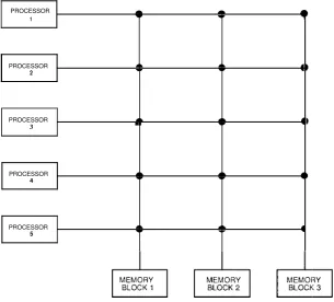
One way to reduce the cost of the decoding circuitry is to divide the shared memory into R blocks, say, of locations each. There are N

+

R two-way lines that allow any processor to gain access to any memory block at any time. However, no more than one processor can read from or write into a block simultaneously. This arrangement is shown in Fig. 1.4 for N = 5 and R = 3. The circles at the intersections of horizontal and vertical lines represent small (relatively inexpensive) switches. When

Figure 1.4 Dividing a shared memory into blocks. PROCESSOR

1

PROCESSOR 2

PROCESSOR

3

..

PROCESSOR 4

(24)

the ith processor wishes to gain access to the jth memory block, it sends its request along the ith horizontal line to the jth switch, which then routes it down the jth vertical line to the jth memory block. Each memory block possesses one decoder circuit to determine which of the locations is needed. Therefore, the total cost of decoding circuitry is R x f To this we must add of course the cost of the N x R switches. Another approach to obtaining a weaker version of the SM SIMD is described in the next section.

1.2.3.2 Interconnection-Network S I M D Computers. We concluded section 1.2.3.1 by showing how the SM SIMD model can be made more feasible by dividing the memory into blocks and making access to these blocks exclusive. It is natural to think of extending this idea to obtain a slightly more powerful model. Here the M locations of the shared memory are distributed among the N processors, each receiving locations. In addition every pair of processors are connected by a two- way line. This arrangement is shown in Fig. 1.5 for N = 5. At any step during the computation, processor can receive a datum from and send another one to (or to Consequently, each processor must contain

(i) a circuit of cost f ( N - 1) capable of decoding a - 1)-bit address-this allows the processor to select one of the other N - 1 processors for communicating; and

(ii) a circuit of cost f capable of decoding a address provided

by another processor.

This model is therefore more powerful than the R-block shared memory, as it allows instantaneous communication between any pair of processors. Several pairs can thus communicate simultaneously (provided, of course, no more than one processor attempts to send data to or expects to receive data from another processor). Thus,

PROCESSOR

Figure 1.5 processors.

(25)

potentially all processors can be busy communicating all the time, something that is not possible in the R-block shared memory when N R. We now discuss a number of features of this model.

(i) Price. The first question to ask is: What is the price paid to fully

interconnect N processors? There are N - 1 lines leaving each processor for a total of N(N - lines. Clearly, such a network is too expensive, especially for large values of N. This is particularly true if we note that with N processors the best we can hope for is an N-fold reduction in the number of steps required by a sequential algorithm, as shown in section 1.3.1.3.

(ii) Feasibility. Even if we could afford such a high price, the model is

unrealistic in practice, again for large values of N. Indeed, there is a limit on the number of lines that can be connected to a processor, and that limit is dictated by the actual physical size of the processor itself.

Relation to S M SIMD. Finally, it should be noted that the fully

interconnected model as described is weaker than a shared-memory computer for the same reason as the R-block shared memory: No more than one processor can gain access simultaneously to the memory block associated with another processor. Allowing the latter would yield a cost of NZ _x_f _{which is about the same as for}

the SM SIMD (not counting the quadratic cost of the two-way lines): This clearly

would defeat our original purpose of getting a more feasible machine!

Simple Networks for SZMD Computers. It is fortunate that in most applications a small subset of all connections is usually sufficient to obtain a good performance. The most popular of these networks are briefly outlined in what follows. Keep in mind that since two processors can communicate in a constant number of steps on a SM SIMD computer, any algorithm for an interconnection-network SIMD

computer can be simulated on the former model in no more steps than required to execute it by the latter.

(i) Linear Array. The simplest way to interconnect N processors is in the form

of a one-dimensional array, as shown in Fig. 1.6 for N = 6. Here, processor is linked to its two neighbors and through a two-way communication line. Each of the end processors, namely, and P,, has only one neighbor.

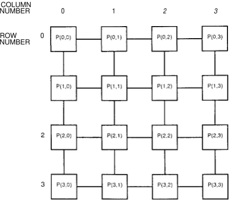
(ii) Two-Dimensional Array. A two-dimensional network is obtained by

arranging the N processors into an m x m array, where m = as shown in Fig. 1.7 for m = 4. The processor in row j and column k is denoted by k), where

j m - 1 and k m - 1. A two-way communication line links k) to its neighbors P ( j

+

1, k), P ( j - k), k

+

and k - 1). Processors on the

(26)

COLUMN

NUMBER 0 1 2 3

ROW 0 NUMBER

Figure 1.7 Two-dimensional array (or mesh) connection.

boundary rows and columns have fewer than four neighbors and hence fewer connections. This network is also known as the mesh.

Both the one- and two-dimensional arrays possess an interesting property: All the lines in the network have the same length. The importance of this feature, not enjoyed by other interconnections studied in this book, will become apparent when we analyze the time required by a network to solve a problem (see section 1.3.4.2).

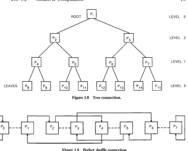
(iii) Tree Connection. In this network, the processors form a complete binary

tree. Such a tree has d levels, numbered to d - 1, and N = - 1 nodes each of which is a processor, as shown in Fig. 1.8 for d = 4. Each processor at level i is connected by a two-way line to its parent at level i

+

1 and to its two children at level

i - 1. The root processor (at level d - 1) has no parent and the leaves (all of which are at level have no children. In this book, the terms tree connection (or tree-connected computer) are used to refer to such a tree of processors.

(iv) Perfect Shuffle Connection. Let N processors

. .

, be

available where N is a power of 2. In the perfect interconnection a one-way line links to where

for 0 i N / 2 - 1,

+

- N for -

as shown in Fig. 1.9 for N = 8. Equivalently, the binary representation of j is obtained by cyclically shifting that of i one position to the left.

In addition to these links, two-way lines connecting every even-numbered processor to its successor are sometimes added to the network. These connections, called the exchange links, are shown as broken lines in Fig. 1.9. In this case, the

(27)

LEVEL 3

LEVEL 2

LEVEL 1

LEAVES

Figure 1.8 Tree connection.

LEVEL

Figure 1.9 Perfect shuffle connection.

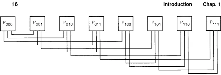
(v) Cube Connection. Assume that N = for some q 1 and let N pro-

cessors be available p , , .

. . ,

,.

A q-dimensional cube (or hypercube) is obtained by connecting each processor to q neighbors. The q neighbors of are defined as follows: The binary representation of j is obtained from that of i by complementing a single bit. This is illustrated in Fig. 1.10 for q = 3. The indices of

. . .

, P, are given in binary notation. Note that each processor has three neighbors.

There are several other interconnection networks besides the ones just described. The decision regarding which of these to use largely depends on the application and in particular on such factors as the kinds of computations to be performed, the desired speed of execution, and the number of processors available. We conclude this section by illustrating a parallel algorithm for an SIMD computer that uses an interconnection network.

Example 1.5

(28)

Figure 1.10 Cube connection.

example 1.1. Using a tree-connected S I M D computer with log levels and leaves, the job can be done in log n steps as shown in Fig. 1.1 1 for = 8.

The original input is a t the leaves, two numbers per leaf. Each leaf adds its inputs and sends the result to its parent. The process is now repeated at each subsequent level: Each processor receives two inputs from its children, computes their sum, and sends it to its parent. The final result is eventually produced by the root. Since at each level ail the processors operate in parallel, the sum is computed in log steps. This compares very favorably with the sequential computation.

The improvement in speed is even more dramatic when m sets, each of n numbers, are available and the sum of each set is to be computed. A conventional machine requires mn steps in this case. A naive application of the parallel algorithm produces them sums in

(29)

n ) steps. Through a process known as pipelining, however, we can do significantly better. Notice that once a set has been processed by the leaves, they are free to receive the next one. The same observation applies to all processors at higher levels. Hence each of the m - 1 sets that follow the initial one can be input to the leaves one step after their predecessor. Once the first sum exits from the root, a new sum is produced in the next step. The entire process therefore takes log n

+

m - 1 steps.

It should be clear from our discussion so far that SIMD computers are considerably more versatile than those conforming to the MISD model. Numerous problems covering a wide variety of applications can be solved by parallel algorithms on SIMD computers. Also, as shown by examples 1.4 and 1.5, algorithms for these computers are relatively easy to design, analyze, and implement. In one respect, however, this class of problems is restricted to those that can be subdivided into a set of identical subproblems all of which are then solved simultaneously by the same set of instructions. Obviously, there are many computations that do not fit this pattern. In some problems it may not be possible or desirable to execute all instructions synchronously. Typically, such problems are subdivided into subproblems that are not necessarily identical and cannot or should not be solved by the same set of instructions. To solve these problems, we turn to the class of MIMD computers.

1.2.4 MIMD Computers

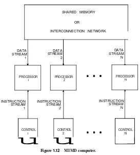
This class of computers is the most general and most powerful in our paradigm of parallel computation that classifies parallel computers according to whether the instruction and/or the data streams are duplicated. Here we have N processors, N streams of instructions, and N streams of data, as shown in Fig. 1.12. The processors here are of the type used in MISD computers in the sense that each possesses its own control unit in addition to its local memory and arithmetic and logic unit. This makes these processors more powerful than the ones used for SIMD computers.

Each processor operates under the control of an instruction stream issued by its control unit. Thus the processors are potentially all executing different programs on different data while solving different subproblems of a single problem. This means that the processors typically operate asynchronously. As with SIMD computers, communication between processors is performed through a shared memory or an interconnection network. MIMD computers sharing a common memory are often referred to as multiprocessors (or tightly coupled machines) while those with an interconnection network are known as multicomputers (or loosely coupled machines).

(30)

Figure 1.12 MIMD computer.

SHARED MEMORY OR

INTERCONNECTION NETWORK

Multicomputers are sometimes referred to as distributed systems. The distinction is usually based on the physical distance separating the processors and is therefore often subjective. A rule of thumb is the following: If all the processors are in close proximity of one another (they are all in the same room, say), then they are a multicomputer; otherwise (they are in different cities, say) they are a distributed system. The nomenclature is relevant only when it comes to evaluating parallel algorithms. Because processors in a distributed system are so far apart, the number of data exchanges among them is significantly more important than the number of computational steps performed by any of them.

The following example examines an application where the great flexibility of MIMD computers is exploited.

Computer programs that play games of strategy, such as chess, do so by generating and searching so-called game trees. The root of the tree is the current game configuration or position from which the program is to make a move. Children of the root represent all the positions reached through one move by the program. Nodes at the next level represent all positions reached through the opponent's reply. This continues up to some predefined

(31)

number of levels. Each leaf position is now assigned a value representing its "goodness" from the program's point of view. The program then determines the path leading to the best position it can reach assuming that the opponent plays a perfect game. Finally, the original move on this path an edge leaving the root) is selected for the program.

As there are typically several moves per position, game trees tend to be very large. In order to cut down on the search time, these trees are generated as they are searched. The idea is to explore the tree using the depth-first search method. From the given root position, paths are created and examined one by one. First, a complete path is built from the root to a leaf. The next path is obtained by backing up from the current leaf to a position all of whose descendants have not yet been explored and building a new path. During the generation of such a path it may happen that a position is reached that, based on information collected so far, definitely leads to leaves that are no better than the ones already examined. In this case the program interrupts its search along that path and all descendants of that position are ignored. A cutoff is said to have occurred. Search can now resume along a new path.

So far we have described the search procedure as it would be executed sequentially. One way to implement it on an MIMD computer would be to distribute the of the root among the processors and let as many as possible be explored in parallel. During the search the processors may exchange various pieces of information. For example, one processor may obtain from another the best move found so far: This may lead to further cutoffs. Another datum that may be communicated is whether a processor has finished searching its If there is a that is still under consideration, then an idle processor may be assigned the job of searching part of that

This approach clearly does not lend itself to implementation on an SIMD computer as the sequence of operations involved in the search is not predictable in advance. At any given point, the instruction being executed varies from one processor to another: While one processor may be generating a new position, a second may be evaluating a leaf, a third may be executing a cutoff, a fourth may be backing up to start a new path, a fifth may be communicating its best move, a sixth may be signaling the end of its search, and so on.

1.2.4.1 Programming MIMD Computers. As mentioned earlier, the M I M D model of parallel computation is the most general and powerful possible. Computers in this class are used to solve in parallel those problems that lack the regular structure required by the SIMD model. This generality does not come for free: Asynchronous algorithms are difficult to design, evaluate, and implement. In order to appreciate the complexity involved in programming M I M D computers, it is important to distinguish between the notion of a process and that of a processor. An asynchronous algorithm is a collection of processes some or all of which are executed simultaneously on a number of available processors. Initially, all processors are free. The parallel algorithm starts its execution on an arbitrarily chosen processor. Shortly thereafter it creates a number of computational tasks, or processes, t o be performed. A process thus corresponds to a section of the algorithm: There may be several processes associated with the same algorithm section, each with a different parameter.

(32)

is available, the process is assigned to the processor that performs the computations specified by the process. Otherwise (if no free processor is available), the process is queued and waits for a processor to be free.

When a processor completes execution of a process, it becomes free. If a process is waiting t o be executed, then it can be assigned to the processor just freed. Otherwise (if no process is waiting), the processor is queued and waits for a process to be created. The order in which processes are executed by processors can obey any policy that assigns priorities to processes. For example, processes can be executed in a in-first-out or in a last-in-first-out order. Also, the availability of a processor is sometimes not sufficient for the processor to be assigned a waiting process. An additional condition may have to be satisfied before the process starts. Similarly, if a processor has already been assigned a process and an unsatisfied condition is encountered during execution, then the processor is freed. When the condition for resumption of that process is later satisfied, a processor (not necessarily the original one) is assigned to it. These are but a few of the scheduling problems that characterize the programming of multiprocessors. Finding efficient solutions to these problems is of paramount importance if MIMD computers are to be considered useful. Note that none of these scheduling problems arise on the less flexible but easier to program SIMD computers.

1.2.4.2 S p e c i a l - P u r p o s e A r c h i t e c t u r e s . In theory, any parallel algorithm can be executed efficiently on the MIMD model. The latter can therefore be used to build parallel computers with a wide variety of applications. Such computers are said to have a general-purpose architecture. In practice, by contrast, it is quite sensible in many applications t o assemble several processors in a configuration specifically designed for the problem at hand. The result is a parallel computer well suited for solving that problem very quickly but that cannot in general be used for any other purpose. Such a computer is said to have a special-purpose architecture. With a particular problem in mind, there are several ways to design a special-purpose parallel computer. For example, a collection of specialized or very simple processors may be used in one of the standard networks such as the mesh. Alternatively, one may interconnect a number of standard processors in a custom geometry. These two approaches may also be combined.

Example 1.7

(33)

1.3 Analyzing Algorithms 21

configuration where each processor is linked to its eight closest neighbors the mesh with diagonal connections in addition to horizontal and vertical ones). Each processor corresponds to a pixel and stores its value. All the processors can now execute the following step in parallel: if a pixel is and all its neighbors are it changes its value to

One final observation is in order in concluding this section. Having studied a variety of approaches to building parallel computers, it is natural to ask: How is one to choose a parallel computer from among the available models? We already saw how one model can use its computational abilities to simulate an algorithm designed for another model. In fact, we shall show in the next section that one processor is capable of executing any parallel algorithm. This indicates that all the models of parallel computers are equivalent in terms of the problems that they can solve. What distinguishes one from another is the ease and speed with which it solves a particular problem. Therefore, the range of applications for which the computer will be used and the urgency with which answers to problems are needed are important factors in deciding what parallel computer to use. However, as with many things in life, the choice of a parallel computer is mostly dictated by economic considerations.

1.3 ANALYZING ALGORITHMS

This book is concerned with two aspects of parallel algorithms: their design and their analysis. A number of algorithm design techniques were illustrated in section 1.2 in connection with our description of the different models of parallel computation. The examples studied therein also dealt with the question of algorithm analysis. This refers to the process of determining how good an algorithm is, that is, how fast, how expensive to run, and how efficient it is in its use of the available resources. In this section we define more formally the various notions used in this book when analyzing parallel algorithms.

Once a new algorithm for some problem has been designed, it is usually evaluated using the following criteria: running time, number of processors used, and cost. Besides these standard metrics, a number of other technology-related measures are sometimes used when it is known that the algorithm is destined to run on a computer based on that particular technology.

1.3.1 Running Time

(34)

equal to the time elapsed between the moment the first processor to begin computing starts and the moment the last processor to end computing terminates.

1.3.1.1 Counting Steps. Before actually implementing an algorithm (whether sequential or parallel) on a computer, it is customary to conduct a theoretical analysis of the time it will require to solve the computational problem at hand. This is usually done by counting the number of basic operations, or steps,

executed by the algorithm in the worst case. This yields an expression describing the number of such steps as a function of the input size. The definition of what constitutes a step varies of course from one theoretical model of computation to another. Intuitively, however, comparing, adding, or swapping two numbers are commonly accepted basic operations in most models. Indeed, each of these operations requires a constant number of time units, or cycles, on a typical (SISD) computer. The running time of a parallel algorithm is usually obtained by counting two kinds of steps:

computational steps and routing steps. A computational step is an arithmetic or logic operation performed on a datum within a processor. In a routing step, on the other hand, a datum travels from one processor to another via the shared memory or through the communication network. For a problem of size n, the parallel worst-case running time of an algorithm, a function of n, will be denoted by Strictly speaking, the running time is also a function of the number of processors. Since the latter can always be expressed as a function of n, we shall write t as a function of the size of the input to avoid complicating our notation.

Example 1.8

In example 1.4 we studied a parallel algorithm that searches a file with n entries on an processor EREW SM SIMD computer. The algorithm requires log N parallel steps to broadcast the value to be searched for and comparison steps within each processor. Assuming that each step (broadcast or comparison) requires one time unit, we say that the algorithms runs in log N

+

time, that is, = log N

+

In general, computational steps and routing steps d o not necessarily require the same number of time units. A routing step usually depends on the distance between the processors and typically takes a little longer to execute than a computational step.

Lower and Upper Bounds. Given a computational problem for which a new sequential algorithm has just been designed, it is common practice among algorithm designers to ask the following two questions:

(i) Is it the fastest possible algorithm for the problem?

(ii) If not, how does it compare with other existing algorithms for the same

problem?

(35)

1.3 Analyzing Algorithms 23

Example 1.9

Say that we want to compute the product of two x matrices. Since the resulting matrix has n2 _{entries, at least this many steps are needed by any matrix multiplication}

algorithm simply to produce the output.

Lower bounds, such as the one in example 1.9, are usually known as obvious or trivial lower bounds, as they are obtained by counting the number of steps needed during input and/or output. A more sophisticated lower bound is derived in the next example.

Example 1.10

The problem of sorting is defined as follows: A set of n numbers in random order is given; arrange the numbers in nondecreasing order. There are n ! possible permutations of the input and log n ! on the order of n log n) bits are needed to distinguish among them. Therefore, in the worst case, any algorithm for sorting requires on the order of log n steps at least to recognize a particular output.

If the number of steps a n algorithm executes in the worst case is equal t o (or of the same order as) the lower bound, then the algorithm is the fastest possible and is said to be optimal. Otherwise, a faster algorithm may have to be invented, or it may be possible t o improve the lower bound. In any case, if the new algorithm is faster than all known algorithms for the problem, then we say that it has established a new upper bound on the number of steps required to solve that problem in the worst case. Question (ii) is therefore always settled by comparing the running time of the new algorithm with the existing upper bound for the problem (established by the fastest previously known algorithm).

Example 1.11

To date, no algorithm is known for multiplying two n x matrices in steps. The standard textbook algorithm requires on the order of n3 _{operations. However, the upper}

bound on this problem is established at the time of this writing by an algorithm requiring on the order of operations at most, where < 2.5.

By contrast, several sorting algorithms exist that require on the order of at most log operations and are hence optimal.

In the preceding discussion, we used the phrase "on the order of" to express lower and upper bounds. We now introduce some notation for that purpose. Let f (n) and be functions from the positive integers to the positive reals:

(i) The function is said to be of order at least f (n), denoted f (n)), if there are positive constants c and such that cf (n) for all n

The function is said to be of order at most f (n), denoted f (n)), if there are positive constants c and such that cf (n) for all n