Algorithms and
Parallel Computing
Fayez Gebali
University of Victoria, Victoria, BC
Copyright © 2011 by John Wiley & Sons, Inc. All rights reserved
Published by John Wiley & Sons, Inc., Hoboken, New Jersey Published simultaneously in Canada No part of this publication may be reproduced, stored in a retrieval system, or transmitted in any form or by any means, electronic, mechanical, photocopying, recording, scanning, or otherwise, except as permitted under Section 107 or 108 of the 1976 United States Copyright Act, without either the prior written permission of the Publisher, or authorization through payment of the appropriate per-copy fee to the Copyright Clearance Center, Inc., 222 Rosewood Drive, Danvers, MA 01923, (978) 750-8400, fax (978) 750-4470, or on the web at www.copyaright.com. Requests to the Publisher for permission should be addressed to the Permissions Department, John Wiley & Sons, Inc., 111 River Street, Hoboken, NJ 07030, (201) 748-6011, fax (201) 748-6008, or online at http://www.wiley.com/go/ permission.
Limit of Liability/Disclaimer of Warranty: While the publisher and author have used their best efforts in preparing this book, they make no representations or warranties with respect to the accuracy or completeness of the contents of this book and specifi cally disclaim any implied warranties of merchantability or fi tness for a particular purpose. No warranty may be created or extended by sales representatives or written sales materials. The advice and strategies contained herein may not be suitable for your situation. You should consult with a professional where appropriate. Neither the publisher nor author shall be liable for any loss of profi t or any other commercial damages, including but not limited to special, incidental, consequential, or other damages.
For general information on our other products and services or for technical support, please contact our Customer Care Department within the United States at (800) 762-2974, outside the United States at (317) 572-3993 or fax (317) 572-4002.
Wiley also publishes its books in a variety of electronic formats. Some content that appears in print may not be available in electronic formats. For more information about Wiley products, visit our web site at www.wiley.com.
Library of Congress Cataloging-in-Publication Data Gebali, Fayez.
Algorithms and parallel computing/Fayez Gebali.
p. cm.—(Wiley series on parallel and distributed computing ; 82) Includes bibliographical references and index.
ISBN 978-0-470-90210-3 (hardback)
1. Parallel processing (Electronic computers) 2. Computer algorithms. I. Title. QA76.58.G43 2011
004′.35—dc22
2010043659 Printed in the United States of America
Contents
Preface xiii
List of Acronyms xix
1 Introduction 1
1.1 Introduction 1
1.2 Toward Automating Parallel Programming 2 1.3 Algorithms 4
1.4 Parallel Computing Design Considerations 12 1.5 Parallel Algorithms and Parallel Architectures 13 1.6 Relating Parallel Algorithm and Parallel Architecture 14 1.7 Implementation of Algorithms: A Two-Sided Problem 14 1.8 Measuring Benefi ts of Parallel Computing 15
1.9 Amdahl’s Law for Multiprocessor Systems 19 1.10 Gustafson–Barsis’s Law 21
1.11 Applications of Parallel Computing 22
2 Enhancing Uniprocessor Performance 29
2.1 Introduction 29
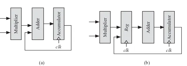
2.2 Increasing Processor Clock Frequency 30 2.3 Parallelizing ALU Structure 30
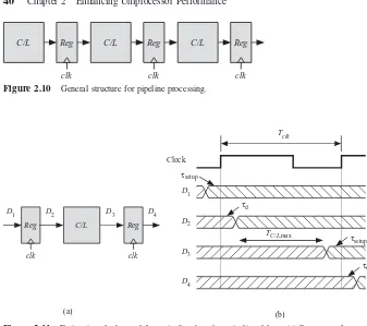
2.4 Using Memory Hierarchy 33 2.5 Pipelining 39
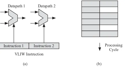
2.6 Very Long Instruction Word (VLIW) Processors 44
2.7 Instruction-Level Parallelism (ILP) and Superscalar Processors 45 2.8 Multithreaded Processor 49
3 Parallel Computers 53
3.1 Introduction 53 3.2 Parallel Computing 53
3.3 Shared-Memory Multiprocessors (Uniform Memory Access [UMA]) 54
3.4 Distributed-Memory Multiprocessor (Nonuniform Memory Access [NUMA]) 56
viii Contents
3.5 SIMD Processors 57 3.6 Systolic Processors 57 3.7 Cluster Computing 60 3.8 Grid (Cloud) Computing 60 3.9 Multicore Systems 61 3.10 SM 62
3.11 Communication Between Parallel Processors 64 3.12 Summary of Parallel Architectures 67
4 Shared-Memory Multiprocessors 69
4.1 Introduction 69
4.2 Cache Coherence and Memory Consistency 70 4.3 Synchronization and Mutual Exclusion 76
5 Interconnection Networks 83
5.1 Introduction 83
5.2 Classifi cation of Interconnection Networks by Logical Topologies 84 5.3 Interconnection Network Switch Architecture 91
6 Concurrency Platforms 105
6.1 Introduction 105
6.2 Concurrency Platforms 105 6.3 Cilk++ 106
6.4 OpenMP 112
6.5 Compute Unifi ed Device Architecture (CUDA) 122
7 Ad Hoc Techniques for Parallel Algorithms 131
7.1 Introduction 131
7.2 Defi ning Algorithm Variables 133 7.3 Independent Loop Scheduling 133 7.4 Dependent Loops 134
7.5 Loop Spreading for Simple Dependent Loops 135 7.6 Loop Unrolling 135
7.7 Problem Partitioning 136
7.8 Divide-and-Conquer (Recursive Partitioning) Strategies 137 7.9 Pipelining 139
8 Nonserial–Parallel Algorithms 143
8.1 Introduction 143
8.2 Comparing DAG and DCG Algorithms 143
Contents ix 8.4 Formal Technique for Analyzing NSPAs 147
8.5 Detecting Cycles in the Algorithm 150
8.6 Extracting Serial and Parallel Algorithm Performance Parameters 151 8.7 Useful Theorems 153
8.8 Performance of Serial and Parallel Algorithms on Parallel Computers 156
9 z-Transform Analysis 159
9.1 Introduction 159
9.2 Defi nition of z-Transform 159
9.3 The 1-D FIR Digital Filter Algorithm 160
9.4 Software and Hardware Implementations of the z-Transform 161 9.5 Design 1: Using Horner’s Rule for Broadcast Input and
Pipelined Output 162
9.6 Design 2: Pipelined Input and Broadcast Output 163 9.7 Design 3: Pipelined Input and Output 164
10 Dependence Graph Analysis 167
10.1 Introduction 167
10.2 The 1-D FIR Digital Filter Algorithm 167 10.3 The Dependence Graph of an Algorithm 168
10.4 Deriving the Dependence Graph for an Algorithm 169 10.5 The Scheduling Function for the 1-D FIR Filter 171 10.6 Node Projection Operation 177
10.7 Nonlinear Projection Operation 179
10.8 Software and Hardware Implementations of the DAG Technique 180
11 Computational Geometry Analysis 185
11.1 Introduction 185
11.2 Matrix Multiplication Algorithm 185
11.3 The 3-D Dependence Graph and Computation Domain D 186 11.4 The Facets and Vertices of D 188
11.5 The Dependence Matrices of the Algorithm Variables 188
11.6 Nullspace of Dependence Matrix: The Broadcast Subdomain B 189 11.7 Design Space Exploration: Choice of Broadcasting versus
Pipelining Variables 192 11.8 Data Scheduling 195
11.9 Projection Operation Using the Linear Projection Operator 200 11.10 Effect of Projection Operation on Data 205
x Contents
12 Case Study: One-Dimensional IIR Digital Filters 209
12.1 Introduction 209
12.2 The 1-D IIR Digital Filter Algorithm 209 12.3 The IIR Filter Dependence Graph 209
12.4 z-Domain Analysis of 1-D IIR Digital Filter Algorithm 216
13 Case Study: Two- and Three-Dimensional Digital Filters 219
13.1 Introduction 219
13.2 Line and Frame Wraparound Problems 219 13.3 2-D Recursive Filters 221
13.4 3-D Digital Filters 223
14 Case Study: Multirate Decimators and Interpolators 227
14.1 Introduction 227
14.2 Decimator Structures 227
14.3 Decimator Dependence Graph 228 14.4 Decimator Scheduling 230 14.5 Decimator DAG for s1= [1 0] 231
14.6 Decimator DAG for s2= [1 −1] 233
14.7 Decimator DAG for s3= [1 1] 235
14.8 Polyphase Decimator Implementations 235 14.9 Interpolator Structures 236
14.10 Interpolator Dependence Graph 237 14.11 Interpolator Scheduling 238 14.12 Interpolator DAG for s1= [1 0] 239
14.13 Interpolator DAG for s2= [1 −1] 241
14.14 Interpolator DAG for s3= [1 1] 243
14.15 Polyphase Interpolator Implementations 243
15 Case Study: Pattern Matching 245
15.1 Introduction 245
15.2 Expressing the Algorithm as a Regular Iterative Algorithm (RIA) 245 15.3 Obtaining the Algorithm Dependence Graph 246
15.4 Data Scheduling 247 15.5 DAG Node Projection 248
15.6 DESIGN 1: Design Space Exploration When s = [1 1]t
249 15.7 DESIGN 2: Design Space Exploration When s = [1 −1]t
252 15.8 DESIGN 3: Design Space Exploration When s = [1 0]t
253
16 Case Study: Motion Estimation for Video Compression 255
Contents xi 16.3 Data Buffering Requirements 257
16.4 Formulation of the FBMA 258
16.5 Hierarchical Formulation of Motion Estimation 259 16.6 Hardware Design of the Hierarchy Blocks 261 17 Case Study: Multiplication over GF(2m)
267
17.1 Introduction 267
17.2 The Multiplication Algorithm in GF(2m
) 268 17.3 Expressing Field Multiplication as an RIA 270 17.4 Field Multiplication Dependence Graph 270 17.5 Data Scheduling 271
17.6 DAG Node Projection 273 17.7 Design 1: Using d1= [1 0]t 275
17.8 Design 2: Using d2= [1 1]t 275
17.9 Design 3: Using d3= [1 −1]t 277
17.10 Applications of Finite Field Multipliers 277
18 Case Study: Polynomial Division over GF(2) 279
18.1 Introduction 279
18.2 The Polynomial Division Algorithm 279 18.3 The LFSR Dependence Graph 281 18.4 Data Scheduling 282
18.5 DAG Node Projection 283
18.6 Design 1: Design Space Exploration When s1= [1 −1] 284
18.7 Design 2: Design Space Exploration When s2= [1 0] 286
18.8 Design 3: Design Space Exploration When s3= [1 −0.5] 289
18.9 Comparing the Three Designs 291
19 The Fast Fourier Transform 293
19.1 Introduction 293
19.2 Decimation-in-Time FFT 295
19.3 Pipeline Radix-2 Decimation-in-Time FFT Processor 298 19.4 Decimation-in-Frequency FFT 299
19.5 Pipeline Radix-2 Decimation-in-Frequency FFT Processor 303
20 Solving Systems of Linear Equations 305
20.1 Introduction 305
20.2 Special Matrix Structures 305
20.3 Forward Substitution (Direct Technique) 309 20.4 Back Substitution 312
20.5 Matrix Triangularization Algorithm 312
xii Contents
21 Solving Partial Differential Equations Using Finite
Difference Method 323
21.1 Introduction 323
21.2 FDM for 1-D Systems 324 References 331
Preface
ABOUT THIS BOOK
There is a software gap between hardware potential and the performance that can be attained using today ’ s software parallel program development tools. The tools need manual intervention by the programmer to parallelize the code. This book is intended to give the programmer the techniques necessary to explore parallelism in algorithms, serial as well as iterative. Parallel computing is now moving from the realm of specialized expensive systems available to few select groups to cover almost every computing system in use today. We can fi nd parallel computers in our laptops, desktops, and embedded in our smart phones. The applications and algo-rithms targeted to parallel computers were traditionally confi ned to weather predic-tion, wind tunnel simulations, computational biology, and signal processing. Nowadays, just about any application that runs on a computer will encounter the parallel processors now available in almost every system.
Parallel algorithms could now be designed to run on special - purpose parallel processors or could run on general - purpose parallel processors using several multi-level techniques such as parallel program development, parallelizing compilers, multithreaded operating systems, and superscalar processors. This book covers the fi rst option: design of special - purpose parallel processor architectures to implement a given class of algorithms. We call such systems accelerator cores. This book forms the basis for a course on design and analysis of parallel algorithms. The course would cover Chapters 1 – 4 then would select several of the case study chapters that consti-tute the remainder of the book.
Although very large - scale integration (VLSI) technology allows us to integrate more processors on the same chip, parallel programming is not advancing to match these technological advances. An obvious application of parallel hardware is to design special - purpose parallel processors primarily intended for use as accelerator cores in multicore systems. This is motivated by two practicalities: the prevalence of multicore systems in current computing platforms and the abundance of simple parallel algorithms that are needed in many systems, such as in data encryption/ decryption, graphics processing, digital signal processing and fi ltering, and many more.
It is simpler to start by stating what this book is not about. This book does not attempt to give a detailed coverage of computer architecture, parallel computers, or algorithms in general. Each of these three topics deserves a large textbook to attempt to provide a good cover. Further, there are the standard and excellent textbooks for each, such as Computer Organization and Design by D.A. Patterson and J.L.
xiv Preface
Hennessy, Parallel Computer Architecture by D.E. Culler, J.P. Singh, and A. Gupta, and fi nally, Introduction to Algorithms by T.H. Cormen, C.E. Leiserson, and R.L. Rivest. I hope many were fortunate enough to study these topics in courses that adopted the above textbooks. My apologies if I did not include a comprehensive list of equally good textbooks on the above subjects.
This book, on the other hand, shows how to systematically design special -purpose parallel processing structures to implement algorithms. The techniques presented here are general and can be applied to many algorithms, parallel or otherwise.
This book is intended for researchers and graduate students in computer engi-neering, electrical engiengi-neering, and computer science. The prerequisites for this book are basic knowledge of linear algebra and digital signal processing. The objectives of this book are (1) to explain several techniques for expressing a parallel algorithm as a dependence graph or as a set of dependence matrices; (2) to explore scheduling schemes for the processing tasks while conforming to input and output data timing, and to be able to pipeline some data and broadcast other data to all processors; and (3) to explore allocation schemes for the processing tasks to processing elements.
CHAPTER ORGANIZATION AND OVERVIEW
Chapter 1 defi nes the two main classes of algorithms dealt with in this book: serial algorithms, parallel algorithms, and regular iterative algorithms. Design consider-ations for parallel computers are discussed as well as their close tie to parallel algorithms. The benefi ts of using parallel computers are quantifi ed in terms of speedup factor and the effect of communication overhead between the processors. The chapter concludes by discussing two applications of parallel computers.
Chapter 2 discusses the techniques used to enhance the performance of a single computer such as increasing the clock frequency, parallelizing the arithmetic and logic unit (ALU) structure, pipelining, very long instruction word (VLIW), supers-calar computing, and multithreading.
Chapter 3 reviews the main types of parallel computers discussed here and includes shared memory, distributed memory, single instruction multiple data stream (SIMD), systolic processors, and multicore systems.
Chapter 4 reviews shared - memory multiprocessor systems and discusses two main issues intimately related to them: cache coherence and process synchronization.
Chapter 5 reviews the types of interconnection networks used in parallel proces-sors. We discuss simple networks such as buses and move on to star, ring, and mesh topologies. More effi cient networks such as crossbar and multistage interconnection networks are discussed.
Preface xv to ensure data integrity and correct timing of task execution. The techniques devel-oped in this book help the programmer toward this goal for serial algorithms and for regular iterative algorithms.
Chapter 7 reviews the ad hoc techniques used to implement algorithms on paral-lel computers. These techniques include independent loop scheduling, dependent loop spreading, dependent loop unrolling, problem partitioning, and divide and -conquer strategies. Pipelining at the algorithm task level is discussed, and the technique is illustrated using the coordinate rotation digital computer (CORDIC) algorithm.
Chapter 8 deals with nonserial – parallel algorithms (NSPAs) that cannot be described as serial, parallel, or serial – parallel algorithms. NSPAs constitute the majority of general algorithms that are not apparently parallel or show a confusing task dependence pattern. The chapter discusses a formal, very powerful, and simple technique for extracting parallelism from an algorithm. The main advantage of the formal technique is that it gives us the best schedule for evaluating the algorithm on a parallel machine. The technique also tells us how many parallel processors are required to achieve maximum execution speedup. The technique enables us to extract important NSPA performance parameters such as work ( W ), parallelism ( P ), and depth ( D ).
Chapter 9 introduces the z- transform technique. This technique is used for studying the implementation of digital fi lters and multirate systems on different parallel processing machines. These types of applications are naturally studied in the z - domain, and it is only natural to study their software and hardware implementa-tion using this domain.
Chapter 10 discusses to construct the dependence graph associated with an iterative algorithm. This technique applies, however, to iterative algorithms that have one, two, or three indices at the most. The dependence graph will help us schedule tasks and automatically allocate them to software threads or hardware processors.
Chapter 11 discusses an iterative algorithm analysis technique that is based on computation geometry and linear algebra concepts. The technique is general in the sense that it can handle iterative algorithms with more than three indices. An example is two - dimensional (2 - D) or three - dimensional (3 - D) digital fi lters. For such algorithms, we represent the algorithm as a convex hull in a multidimensional space and associate a dependence matrix with each variable of the algorithm. The null space of these matrices will help us derive the different parallel software threads and hardware processing elements and their proper timing.
Chapter 12 explores different parallel processing structures for one - dimensional (1 - D) fi nite impulse response (FIR) digital fi lters. We start by deriving possible hardware structures using the geometric technique of Chapter 11 . Then, we explore possible parallel processing structures using the z - transform technique of Chapter 9 .
Chapter 13 explores different parallel processing structures for 2 - D and 3 - D infi nite impulse response (IIR) digital fi lters. We use the z - transform technique for this type of fi lter.
xvi Preface
especially telecommunications. We use the dependence graph technique of Chapter 10 to derive different parallel processing structures.
Chapter 15 explores different parallel processing structures for the pattern matching problem. We use the dependence graph technique of Chapter 10 to study this problem.
Chapter 16 explores different parallel processing structures for the motion estimation algorithm used in video data compression. In order to delay with this complex algorithm, we use a hierarchical technique to simplify the problem and use the dependence graph technique of Chapter 10 to study this problem.
Chapter 17 explores different parallel processing structures for fi nite - fi eld multiplication over GF (2 m
). The multi - plication algorithm is studied using the dependence graph technique of Chapter 10 .
Chapter 18 explores different parallel processing structures for fi nite - fi eld poly-nomial division over GF (2). The division algorithm is studied using the dependence graph technique of Chapter 10 .
Chapter 19 explores different parallel processing structures for the fast Fourier transform algorithm. Pipeline techniques for implementing the algorithm are reviewed.
Chapter 20 discusses solving systems of linear equations. These systems could be solved using direct and indirect techniques. The chapter discusses how to paral-lelize the forward substitution direct technique. An algorithm to convert a dense matrix to an equivalent triangular form using Givens rotations is also studied. The chapter also discusses how to parallelize the successive over - relaxation (SOR) indi-rect technique.
Chapter 21 discusses solving partial differential equations using the fi nite dif-ference method (FDM). Such equations are very important in many engineering and scientifi c applications and demand massive computation resources.
ACKNOWLEDGMENTS
I wish to express my deep gratitude and thank Dr. M.W. El - Kharashi of Ain Shams University in Egypt for his excellent suggestions and encouragement during the preparation of this book. I also wish to express my personal appreciation of each of the following colleagues whose collaboration contributed to the topics covered in this book:
Dr. Esam Abdel - Raheem Dr. Turki Al - Somani
University of Windsor, Canada Al - Baha University, Saudi Arabia Dr. Atef Ibrahim Dr. Mohamed Fayed
Electronics Research Institute, Egypt Al - Azhar University, Egypt Mr. Brian McKinney Dr. Newaz Rafi q
ICEsoft, Canada ParetoLogic, Inc., Canada Dr. Mohamed Rehan Dr. Ayman Tawfi k
Preface xvii
COMMENTS AND SUGGESTIONS
This book covers a wide range of techniques and topics related to parallel comput-ing. It is highly probable that it contains errors and omissions. Other researchers and/or practicing engineers might have other ideas about the content and organiza-tion of a book of this nature. We welcome receiving comments and suggesorganiza-tions for consideration. If you fi nd any errors, we would appreciate hearing from you. We also welcome ideas for examples and problems (along with their solutions if pos-sible) to include with proper citation.
Please send your comments and bug reports electronically to [email protected] , or you can fax or mail the information to
Dr. F ayez G ebali
Electrical and Computer Engineering Department University of Victoria, Victoria, B.C., Canada V8W 3P6 Tel: 250 - 721 - 6509
List of Acronyms
1 - D one - dimensional 2 - D two - dimensional 3 - D three - dimensional ALU arithmetic and logic unit
AMP asymmetric multiprocessing system API application program interface ASA acyclic sequential algorithm
ASIC application - specifi c integrated circuit ASMP asymmetric multiprocessor
CAD computer - aided design CFD computational fl uid dynamics CMP chip multiprocessor
CORDIC coordinate rotation digital computer CPI clock cycles per instruction
CPU central processing unit CRC cyclic redundancy check CT computerized tomography
CUDA compute unifi ed device architecture DAG directed acyclic graph
DBMS database management system DCG directed cyclic graph
DFT discrete Fourier transform DG directed graph
DHT discrete Hilbert transform DRAM dynamic random access memory DSP digital signal processing
FBMA full - search block matching algorithm FDM fi nite difference method
FDM frequency division multiplexing FFT fast Fourier transform
FIR fi nite impulse response
FLOPS fl oating point operations per second FPGA fi eld - programmable gate array GF(2 m
) Galois fi eld with 2 m
elements
GFLOPS giga fl oating point operations per second GPGPU general purpose graphics processor unit GPU graphics processing unit
xx List of Acronyms
HCORDIC high - performance coordinate rotation digital computer HDL hardware description language
HDTV high - defi nition TV
HRCT high - resolution computerized tomography HTM hardware - based transactional memory IA iterative algorithm
IDHT inverse discrete Hilbert transform
IEEE Institute of Electrical and Electronic Engineers IIR infi nite impulse response
ILP instruction - level parallelism I/O input/output
IP intellectual property modules IP Internet protocol
IR instruction register ISA instruction set architecture JVM Java virtual machine LAN local area network LCA linear cellular automaton LFSR linear feedback shift register LHS left - hand side
LSB least - signifi cant bit MAC medium access control MAC multiply/accumulate
MCAPI Multicore Communications Management API MIMD multiple instruction multiple data
MIMO multiple - input multiple - output MIN multistage interconnection networks MISD multiple instruction single data stream MIMD multiple instruction multiple data MPI message passing interface
MRAPI Multicore Resource Management API MRI magnetic resonance imaging
MSB most signifi cant bit
MTAPI Multicore Task Management API
NIST National Institute for Standards and Technology NoC network - on - chip
NSPA nonserial – parallel algorithm NUMA nonuniform memory access NVCC NVIDIA C compiler
OFDM orthogonal frequency division multiplexing OFDMA orthogonal frequency division multiple access OS operating system
List of Acronyms xxi PRAM parallel random access machine
QoS quality of service
RAID redundant array of inexpensive disks RAM random access memory
RAW read after write RHS right - hand side
RIA regular iterative algorithm RTL register transfer language SE switching element SF switch fabric SFG signal fl ow graph
SIMD single instruction multiple data stream SIMP single instruction multiple program SISD single instruction single data stream SLA service - level agreement
SM streaming multiprocessor SMP symmetric multiprocessor SMT simultaneous multithreading SoC system - on - chip
SOR successive over - relaxation SP streaming processor SPA serial – parallel algorithm
SPMD single program multiple data stream SRAM static random access memory STM software - based transactional memory TCP transfer control protocol
TFLOPS tera fl oating point operations per second TLP thread - level parallelism
TM transactional memory UMA uniform memory access
VHDL very high - speed integrated circuit hardware description language VHSIC very high - speed integrated circuit
VIQ virtual input queuing VLIW very long instruction word VLSI very large - scale integration VOQ virtual output queuing VRQ virtual routing/virtual queuing WAN wide area network
Chapter
1
Introduction
1.1 INTRODUCTION
The idea of a single - processor computer is fast becoming archaic and quaint. We now have to adjust our strategies when it comes to computing:
• It is impossible to improve computer performance using a single processor. Such processor would consume unacceptable power. It is more practical to use many simple processors to attain the desired performance using perhaps thousands of such simple computers [1] .
• As a result of the above observation, if an application is not running fast on a single - processor machine, it will run even slower on new machines unless it takes advantage of parallel processing.
• Programming tools that can detect parallelism in a given algorithm have to be developed. An algorithm can show regular dependence among its vari-ables or that dependence could be irregular. In either case, there is room for speeding up the algorithm execution provided that some subtasks can run concurrently while maintaining the correctness of execution can be assured.
• Optimizing future computer performance will hinge on good parallel pro-gramming at all levels: algorithms, program development, operating system, compiler, and hardware.
• The benefi ts of parallel computing need to take into consideration the number of processors being deployed as well as the communication overhead of processor - to - processor and processor - to - memory. Compute - bound problems are ones wherein potential speedup depends on the speed of execution of the algorithm by the processors. Communication - bound problems are ones wherein potential speedup depends on the speed of supplying the data to and extracting the data from the processors.
• Memory systems are still much slower than processors and their bandwidth is limited also to one word per read/write cycle.
Algorithms and Parallel Computing, by Fayez Gebali Copyright © 2011 John Wiley & Sons, Inc.
2 Chapter 1 Introduction
• Scientists and engineers will no longer adapt their computing requirements to the available machines. Instead, there will be the practical possibility that they will adapt the computing hardware to solve their computing requirements.
This book is concerned with algorithms and the special - purpose hardware structures that execute them since software and hardware issues impact each other. Any soft-ware program ultimately runs and relies upon the underlying hardsoft-ware support provided by the processor and the operating system. Therefore, we start this chapter with some defi nitions then move on to discuss some relevant design approaches and design constraints associated with this topic.
1.2 TOWARD AUTOMATING PARALLEL PROGRAMMING
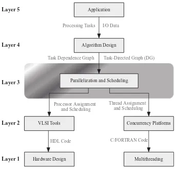
We are all familiar with the process of algorithm implementation in software. When we write a code, we do not need to know the details of the target computer system since the compiler will take care of the details. However, we are steeped in think-ing in terms of a sthink-ingle central processthink-ing unit (CPU) and sequential processthink-ing when we start writing the code or debugging the output. On the other hand, the processes of implementing algorithms in hardware or in software for parallel machines are more related than we might think. Figure 1.1 shows the main phases or layers of implementing an application in software or hardware using parallel computers. Starting at the top, layer 5 is the application layer where the application or problem to be implemented on a parallel computing platform is defi ned. The specifi cations of inputs and outputs of the application being studied are also defi ned. Some input/output (I/O) specifi cations might be concerned with where data is stored and the desired timing relations of data. The results of this layer are fed to the lower layer to guide the algorithm development.
Layer 4 is algorithm development to implement the application in question. The computations required to implement the application defi ne the tasks of the algorithm and their interdependences. The algorithm we develop for the application might or might not display parallelism at this state since we are traditionally used to linear execution of tasks. At this stage, we should not be concerned with task timing or task allocation to processors. It might be tempting to decide these issues, but this is counterproductive since it might preclude some potential parallelism. The result of this layer is a dependence graph, a directed graph (DG), or an adjacency matrix that summarize the task dependences.
1.2 Toward Automating Parallel Programming 3
Layer 2 is the coding layer where the parallel algorithm is coded using a high - level language. The language used depends on the target parallel computing platform. The right branch in Fig. 1.1 is the case of mapping the algorithm on a general - purpose parallel computing platform. This option is really what we mean by
parallel programming . Programming parallel computers is facilitated by what is called concurrency platforms , which are tools that help the programmer manage the threads and the timing of task execution on the processors. Examples of concurrency platforms include Cilk + + , openMP, or compute unifi ed device architecture (CUDA), as will be discussed in Chapter 6 .
The left branch in Fig. 1.1 is the case of mapping the algorithm on a custom parallel computer such as systolic arrays. The programmer uses hardware description language (HDL) such as Verilog or very high - speed integrated circuit hardware (VHDL).
Figure 1.1 The phases or layers of implementing an application in software or hardware using parallel computers.
Layer 5
Parallelization and Scheduling
VLSI Tools Concurrency Platforms
Application
Algorithm Design
Layer 4
Layer 3
Layer 2
I/O Data
Task-Directed Graph (DG)
Thread Assignment and Scheduling Processor Assignment
and Scheduling
Hardware Design Multithreading
Custom Hardware Implementation Software Implementation
Layer 1
Processing Tasks
Task Dependence Graph
4 Chapter 1 Introduction
Layer 1 is the realization of the algorithm or the application on a parallel com-puter platform. The realization could be using multithreading on a parallel comcom-puter platform or it could be on an application - specifi c parallel processor system using application - specifi c integrated circuits (ASICs) or fi eld - programmable gate array (FPGA).
So what do we mean by automatic programming of parallel computers? At the moment, we have automatic serial computer programming. The programmer writes a code in a high - level language such as C, Java, or FORTRAN, and the code is compiled without further input from the programmer. More signifi cantly, the pro-grammer does not need to know the hardware details of the computing platform. Fast code could result even if the programmer is unaware of the memory hierarchy, CPU details, and so on.
Does this apply to parallel computers? We have parallelizing compilers that look for simple loops and spread them among the processors. Such compilers could easily tackle what is termed embarrassingly parallel algorithms [2, 3] . Beyond that, the programmer must have intimate knowledge of how the processors interact among each and when the algorithm tasks are to be executed.
1.3 ALGORITHMS
The IEEE Standard Dictionary of Electrical and Electronics Terms defi nes an algorithm as “ A prescribed set of well - defi ned rules or processes for the solution of a problem in a fi nite number of steps ” [4] . The tasks or processes of an algorithm are interdependent in general. Some tasks can run concurrently in parallel and some must run serially or sequentially one after the other. According to the above defi ni-tion, any algorithm is composed of a serial part and a parallel part. In fact, it is very hard to say that one algorithm is serial while the other is parallel except in extreme trivial cases. Later, we will be able to be more quantitative about this. If the number of tasks of the algorithm is W , then we say that the work associated with the algo-rithm is W .
The basic components defi ning an algorithm are
1. the different tasks,
2. the dependencies among the tasks where a task output is used as another task ’ s input,
3. the set of primary inputs needed by the algorithm, and
4. the set of primary outputs produced by the algorithm.
1.3.1 Algorithm DG
1.3 Algorithms 5
variables fl ow as data between the tasks as indicated by the arrows of the DG. On the other hand, a dependence graph is a graph that has no arrows at its edges, and it becomes hard to fi gure out the data dependencies.
Defi nition 1.1 A dependence graph is a set of nodes and edges. The nodes repre-sent the tasks to be done by the algorithm and the edges reprerepre-sent the data used by the tasks. This data could be input, output, or internal results.
Note that the edges in a dependence graph are undirected since an edge con-necting two nodes does not indicate any input or output data dependency. An edge merely shows all the nodes that share a certain instance of the algorithm variable. This variable could be input, output, or I/O representing intermediate results.
Defi nition 1.2 A DG is a set of nodes and directed edges. The nodes represent the tasks to be done by the algorithm, and the directed edges represent the data depen-dencies among the tasks. The start of an edge is the output of a task and the end of an edge the input to the task.
Defi nition 1.3 A directed acyclic graph (DAG) is a DG that has no cycles or loops. Figure 1.2 shows an example of representing an algorithm by a DAG. A DG or DAG has three types of edges depending on the sources and destinations of the edges.
Defi nition 1.4 An input edge in a DG is one that terminates on one or more nodes but does not start from any node. It represents one of the algorithm inputs.
Referring to Fig. 1.2 , we note that the algorithm has three input edges that represent the inputs in 0 , in 1 , and in 2 .
Defi nition 1.5 An output edge in a DG is one that starts from a node but does not terminate on any other node. It represents one of the algorithm outputs.
Figure 1.2 Example of a directed acyclic graph (DAG) for an algorithm.
1
0 2
4
3
6 5
7 8
9
in0 in1 in2
6 Chapter 1 Introduction
Referring to Fig. 1.2 , we note that the algorithm has three output edges that represent the outputs out 0 , out 1 , and out 2 .
Defi nition 1.6 An internal edge in a DG is one that starts from a node and terminate one or more nodes. It represents one of the algorithm internal variables.
Defi nition 1.7 An input node in a DG is one whose incoming edges are all input edges.
Referring to Fig. 1.2 , we note that nodes 0, 1, and 2 represent input nodes. The tasks associated with these nodes can start immediately after the inputs are available.
Defi nition 1.8 An output node in a DG is whose outgoing edges are all output edges.
Referring to Fig. 1.2 , we note that nodes 7 and 9 represent output nodes. Node 3 in the graph of Fig. 1.2 is not an output node since one of its outgoing edges is an internal edge terminating on node 7.
Defi nition 1.9 An internal node in a DG is one that has at least one incoming internal edge and at least one outgoing internal edge.
1.3.2 Algorithm Adjacency Matrix A
An algorithm could also be represented algebraically as an adjacency matrix A . Given W nodes/tasks, we defi ne the 0 – 1 adjacency matrix A , which is a square
W × W matrix defi ned so that element a ( i , j ) = 1 indicates that node i depends on the output from node j . The source node is j and the destination node is i . Of course, we must have a ( i , i ) = 0 for all values of 0 ≤ i < W since node i does not depend on its own output (self loop), and we assumed that we do not have any loops. The defi -nition of the adjacency matrix above implies that this matrix is asymmetric. This is because if node i depends on node j , then the reverse is not true when loops are not allowed.
As an example, the adjacency matrix for the algorithm in Fig. 1.2 is given by
1.3 Algorithms 7 Matrix A has some interesting properties related to our topic. An input node i is associated with row i , whose elements are all zeros. An output node j is associated with column j , whose elements are all zeros. We can write
Input nodei a i j
All other nodes are internal nodes. Note that all the elements in rows 0, 1, and 2 are all zeros since nodes 0, 1, and 2 are input nodes. This is indicated by the bold entries in these three rows. Note also that all elements in columns 7 and 9 are all zeros since nodes 7 and 9 are output nodes. This is indicated by the bold entries in these two columns. All other rows and columns have one or more nonzero elements to indicate internal nodes. If node i has element a ( i , j ) = 1, then we say that node j is a parent of node i .
1.3.3 Classifying Algorithms Based On Task Dependences
Algorithms can be broadly classifi ed based on task dependences:
The last category could be thought of as a generalization of SPAs. It should be mentioned that the level of data or task granularity can change the algorithm from one class to another. For example, adding two matrices could be an example of a serial algorithm if our basic operation is adding two matrix elements at a time. However, if we add corresponding rows on different computers, then we have a row - based parallel algorithm.
We should also mention that some algorithms can contain other types of algo-rithms within their tasks. The simple matrix addition example serves here as well. Our parallel matrix addition algorithm adds pairs of rows at the same time on dif-ferent processors. However, each processor might add the rows one element at a time, and thus, the tasks of the parallel algorithm represent serial row add algorithms. We discuss these categories in the following subsections.
1.3.4 Serial Algorithms
8 Chapter 1 Introduction
like a long string or queue of dependent tasks. Figure 1.3 a shows an example of a serial algorithm. The algorithm shown is for calculating Fibonnaci numbers. To cal-culate Fibonacci number n 10 , task T 10 performs the following simple calculation:
n10=n8+n9, (1.4) with n 0 = 0 and n 1 = 1 given as initial conditions. Clearly, we can fi nd a Fibonacci
number only after the preceding two Fibonacci numbers have been calculated.
1.3.5 Parallel Algorithms
A parallel algorithm is one where the tasks could all be performed in parallel at the same time due to their data independence. The DG associated with such an algorithm looks like a wide row of independent tasks. Figure 1.3 b shows an example of a parallel algorithm. A simple example of such a purely parallel algorithm is a web server where each incoming request can be processed independently from other requests. Another simple example of parallel algorithms is multitasking in operating systems where the operating system deals with several applications like a web browser, a word processor, and so on.
1.3.6 SPA s
An SPA is one where tasks are grouped in stages such that the tasks in each stage can be executed concurrently in parallel and the stages are executed sequentially. An SPA becomes a parallel algorithm when the number of stages is one. A serial parallel algorithm also becomes a serial algorithm when the number of tasks in each stage is one. Figure 1.3 c shows an example of an SPA. An example of an SPA is the CORDIC algorithm [5 – 8] . The algorithm requires n iterations and at iteration i , three operations are performed:
Figure 1.3 Example of serial, parallel, and serial – parallel algorithms. (a) Serial algorithm. (b) Parallel algorithm. (c) Serial – parallel algorithm.
T0 T1 T2 T3 T4 T5 T6 T7 T8 T9 T10Out
In
(a)
T0 T1 T2 T3 T4 T5
(b) in0
out0 in1
out1 in2
out2 in3
out3 in4
out4 in5
out5 In
(c)
1.3 Algorithms 9
constants that are stored in lookup tables. The parameter m is a control parameter that determines the type of calculations required. The variable θ i is determined before
the start of each iteration. The algorithm performs other operations during each iteration, but we are not concerned about this here. More details can be found in Chapter 7 and in the cited references.
1.3.7 NSPA s
An NSPA does not conform to any of the above classifi cations. The DG for such an algorithm has no pattern. We can further classify NSPA into two main categories based on whether their DG contains cycles or not. Therefore, we can have two types of graphs for NSPA: DCG algorithm. The DCG is most commonly encountered in discrete time feedback control systems. The input is supplied to task T 0 for prefi ltering or input signal
conditioning. Task T 1 accepts the conditioned input signal and the conditioned
feed-back output signal. The output of task T 1 is usually referred to as the error signal,
and this signal is fed to task T 2 to produce the output signal.
Figure 1.4 Example directed graphs for nonserial – parallel algorithms. (a) Directed acyclic graph (DAG). (b) Directed cyclic graph (DCG).
10 Chapter 1 Introduction
The NSPA graph is characterized by two types of constructs: the nodes , which describe the tasks comprising the algorithm, and the directed edges , which describe the direction of data fl ow among the tasks. The lines exiting a node represent an output, and when they enter a node, they represent an input. If task T i produces an
output that is used by task T j , then we say that T j depends on T i . On the graph, we
have an arrow from node i to node j .
The DG of an algorithm gives us three important properties:
1. Work ( W ) , which describes the amount of processing work to be done to complete the algorithm
2. Depth ( D ) , which is also known as the critical path . Depth is defi ned as the maximum path length between any input node and any output node.
3. Parallelism ( P ) , which is also known as the degree of parallelism of the algorithm. Parallelism is defi ned as the maximum number of nodes that can be processed in parallel. The maximum number of parallel processors that could be active at any given time will not exceed B since anymore processors will not fi nd any tasks to execute.
A more detailed discussion of these properties and how an algorithm can be mapped onto a parallel computer is found in Chapter 8 .
1.3.8 RIA s
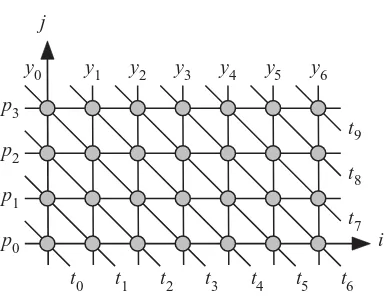
Karp et al. [9, 10] introduced the concept of RIA. This class of algorithms deserves special attention because they are found in algorithms from diverse fi elds such as signal, image and video processing, linear algebra applications, and numerical simu-lation applications that can be implemented in grid structures. Figure 1.5 shows the
dependence graph of a RIA. The example is for pattern matching algorithm. Notice that for a RIA, we do not draw a DAG; instead, we use the dependence graph concept.
Figure 1.5 Dependence graph of a RIA for the pattern matching algorithm.
y0 y1 y2 y3 y4 y5 y6
t0 t1 t2 t3 t4 t5 t6
t7 t8 t9
p0 p1 p2 p3
j
1.3 Algorithms 11 A dependence graph is like a DAG except that the links are not directed and the graph is obtained according to the methodology explained in Chapters 9 , 10 , and 11 .
In a RIA, the dependencies among the tasks show a fi xed pattern. It is a trivial problem to parallelize a serial algorithm, a parallel algorithm, or even an SPA. It is not trivial to explore the possible parallelization options of a RIA. In fact, Chapters 9 – 11 are dedicated to just exploring the parallelization of this class of algorithms.
A simple example of a RIA is the matrix – matrix multiplication algorithm given by Algorithm 1.1.
Algorithm 1.1 Matrix – matrix multiplication algorithm.
Require: Input: matrices A and B
1: for i = 0 : I − 1 do
2: for j = 0 : J − 1 do
3: temp = 0
4: for k = 0 : K − 1 do
5: temp = temp + A ( i , k ) × B ( k , j )
6: end for
7: C ( i , j ) = temp
8: end for
9: end for
10: RETURN C
The variables in the RIA described by Algorithm 1.1 show regular dependence on the algorithm indices i , j, and k. Traditionally, such algorithms are studied using the dependence graph technique, which shows the links between the different tasks to be performed [10 – 12] . The dependence graph is attractive when the number of algorithm indices is 1 or 2. We have three indices in our matrix – matrix multiplication algorithm. It would be hard to visualize such an algorithm using a three dimensional (3 - D) graph. For higher dimensionality algorithms, we use more formal techniques as will be discussed in this book. Chapters 9 – 11 are dedicated to studying such algorithms.
1.3.9 Implementing Algorithms on Parallel Computing
12 Chapter 1 Introduction Serial Algorithms
Serial algorithms, as exemplifi ed by Fig. 1.3 a, cannot be parallelized since the tasks must be executed sequentially. The only parallelization possible is when each task is broken down into parallelizable subtasks. An example is to perform bit - parallel add/multiply operations.
Parallel Algorithms
Parallel algorithms, as exemplifi ed by Fig. 1.3 b, are easily parallelized since all the tasks can be executed in parallel, provided there are enough computing resources. SPA s
SPAs, as exemplifi ed by Fig. 1.3 c, are parallelized by assigning each task in a stage to a software thread or hardware processing element. The stages themselves cannot be parallelized since they are serial in nature.
NSPA s
Techniques for parallelizing NSPAs will be discussed in Chapter 8 . RIA s
Techniques for parallelizing RIAs will be discussed in Chapters 9 – 11 .
1.4 PARALLEL COMPUTING DESIGN CONSIDERATIONS
This section discusses some of the important aspects of the design of parallel com-puting systems. The design of a parallel comcom-puting system requires considering many design options. The designer must choose a basic processor architecture that is capable of performing the contemplated tasks. The processor could be a simple element or it could involve a superscalar processor running a multithreaded operat-ing system.
The processors must communicate among themselves using some form of an
interconnection network . This network might prove to be a bottleneck if it cannot support simultaneous communication between arbitrary pairs of processors. Providing the links between processors is like providing physical channels in tele-communications. How data are exchanged must be specifi ed. A bus is the simplest form of interconnection network. Data are exchanged in the form of words, and a system clock informs the processors when data are valid. Nowadays, buses are being replaced by networks - on - chips (NoC) [13] . In this architecture, data are exchanged on the chip in the form of packets and are routed among the chip modules using
routers .
1.5 Parallel Algorithms and Parallel Architectures 13 the processors or of dedicating a memory module to each processor. When proces-sors need to share data, mechanisms have to be devised to allow reading and writing data in the different memory modules. The order of reading and writing will be important to ensure data integrity. When a shared data item is updated by one pro-cessor, all other processors must be somehow informed of the change so they use the appropriate data value.
Implementing the tasks or programs on a parallel computer involves several design options also. Task partitioning breaks up the original program or application into several segments to be allocated to the processors. The level of partitioning determines the workload allocated to each processor. Coarse grain partitioning allocates large segments to each processor. Fine grain partitioning allocates smaller segments to each processor. These segments could be in the form of separate soft-ware processes or threads . The programmer or the compiler might be the two entities that decide on this partitioning. The programmer or the operating system must ensure proper synchronization among the executing tasks so as to ensure program correct-ness and data integrity.
1.5 PARALLEL ALGORITHMS AND PARALLEL ARCHITECTURES
Parallel algorithms and parallel architectures are closely tied together. We cannot think of a parallel algorithm without thinking of the parallel hardware that will support it. Conversely, we cannot think of parallel hardware without thinking of the parallel software that will drive it. Parallelism can be imple-mented at different levels in a computing system using hardware and software techniques:
1. Data - level parallelism , where we simultaneously operate on multiple bits of a datum or on multiple data. Examples of this are bit - parallel addition mul-tiplication and division of binary numbers, vector processor arrays and sys-tolic arrays for dealing with several data samples. This is the subject of this book.
2. Instruction - level parallelism (ILP) , where we simultaneously execute more than one instruction by the processor. An example of this is use of instruction pipelining.
3. Thread - level parallelism (TLP). A thread is a portion of a program that shares processor resources with other threads. A thread is sometimes called a light-weight process. In TLP, multiple software threads are executed simultane-ously on one processor or on several processors.
14 Chapter 1 Introduction
1.6 RELATING PARALLEL ALGORITHM AND PARALLEL ARCHITECTURE
The IEEE Standard Dictionary of Electrical and Electronics Terms [4] defi nes “ par-allel ” for software as “ simultaneous transfer, occurrence, or processing of the indi-vidual parts of a whole, such as the bits of a character and the characters of a word using separate facilities for the various parts. ” So in that sense, we say an algorithm is parallel when two or more parts of the algorithms can be executed independently on hardware. Thus, the defi nition of a parallel algorithm presupposes availability of supporting hardware. This gives a hint that parallelism in software is closely tied to the hardware that will be executing the software code. Execution of the parts can be done using different threads or processes in the software or on different processors in the hardware. We can quickly identify a potentially parallel algorithm when we see the occurrence of “ FOR ” or “ WHILE ” loops in the code.
On the other hand, the defi nition of parallel architecture, according to The IEEE Standard Dictionary of Electrical and Electronics Terms [4] , is “ a multi - processor architecture in which parallel processing can be performed. ” It is the job of the programmer, compiler, or operating system to supply the multiprocessor with tasks to keep the processors busy. We fi nd ready examples of parallel algorithms in fi elds such as
• scientifi c computing, such as physical simulations, differential equations solvers, wind tunnel simulations, and weather simulation;
• computer graphics, such as image processing, video compression; and ray tracing; and,
• medical imaging, such as in magnetic resonance imaging (MRI) and comput-erized tomography (CT).
There are, however, equally large numbers of algorithms that are not recogniz-ably parallel especially in the area of information technology such as online medical data, online banking, data mining, data warehousing, and database retrieval systems. The challenge is to develop computer architectures and software to speed up the different information technology applications.
1.7 IMPLEMENTATION OF ALGORITHMS: A TWO - SIDED PROBLEM
1.8 Measuring Benefi ts of Parallel Computing 15
Route B represents the classic case when we are given a parallel architecture or a multicore system and we explore the best way to implement a given algorithm on the system subject again to some performance requirements and certain system constraints. In other words, the problem is given a parallel architecture, how can we allocate the different tasks of the parallel algorithm to the different processors? This is the realm of parallel programming using the multithreading design technique. It is done by the application programmer, the software compiler, and the operating system.
Moving along routes A or B requires dealing with
1. mapping the tasks to different processors,
2. scheduling the execution of the tasks to conform to algorithm data depen-dency and data I/O requirements, and
3. identifying the data communication between the processors and the I/O.
1.8 MEASURING BENEFITS OF PARALLEL COMPUTING
We review in this section some of the important results and benefi ts of using parallel computing. But fi rst, we identify some of the key parameters that we will be study-ing in this section.
1.8.1 Speedup Factor
The potential benefi t of parallel computing is typically measured by the time it takes to complete a task on a single processor versus the time it takes to complete the same task on N parallel processors. The speedup S ( N ) due to the use of N parallel processors is defi ned by
S N T T N
p
p
( ) ( )
( ),
= 1 (1.6)
where T p (1) is the algorithm processing time on a single processor and T p ( N ) is
the processing time on the parallel processors. In an ideal situation, for a fully
Figure 1.6 The two paths relating parallel algorithms and parallel architectures.
Algorithm Space
Parallel Computer Space Route A
16 Chapter 1 Introduction
parallelizable algorithm, and when the communication time between processors and memory is neglected , we have T p ( N ) = T p (1)/ N , and the above equation gives
S N( )=N. (1.7) It is rare indeed to get this linear increase in computation domain due to several factors, as we shall see in the book.
1.8.2 Communication Overhead
For single and parallel computing systems, there is always the need to read data from memory and to write back the results of the computations. Communication with the memory takes time due to the speed mismatch between the processor and the memory [14] . Moreover, for parallel computing systems, there is the need for communication between the processors to exchange data. Such exchange of data involves transferring data or messages across the interconnection network.
Communication between processors is fraught with several problems:
1. Interconnection network delay. Transmitting data across the interconnection network suffers from bit propagation delay, message/data transmission delay, and queuing delay within the network. These factors depend on the network topology, the size of the data being sent, the speed of operation of the network, and so on.
2. Memory bandwidth. No matter how large the memory capacity is, access to memory contents is done using a single port that moves one word in or out of the memory at any give memory access cycle.
3. Memory collisions , where two or more processors attempt to access the same memory module. Arbitration must be provided to allow one processor to access the memory at any given time.
4. Memory wall. The speed of data transfer to and from the memory is much slower than processing speed. This problem is being solved using memory hierarchy such as
register↔cache↔RAM↔electronic disk↔magnetic disk↔optic disk To process an algorithm on a parallel processor system, we have several delays as explained in Table 1.1 .
1.8.3 Estimating Speedup Factor and Communication Overhead
1.8 Measuring Benefi ts of Parallel Computing 17
interprocessor communication due to the task independence. We can write under ideal circumstances
Tp( )1 = τN p (1.8) T Np( )= τp. (1.9) The time needed to read the algorithm input data by a single processor is given by Tr( )1 = τN m, (1.10) where τ m is memory access time to read one block of data. We assumed in the above
equation that each task requires one block of input data and N tasks require to read
N blocks. The time needed by the parallel processors to read data from memory is estimated as
T Nr( )=αTr( )1 =α τN m, (1.11) where α is a factor that takes into account limitations of accessing the shared memory. α = 1/ N when each processor maintains its own copy of the required data. α = 1 when data are distributed to each task in order from a central memory. In the worst case, we could have α > N when all processors request data and collide with each other. We could write the above observations as
T Nr N
m
m ( )
= =
τ τ
when Distributed memory
when Shared memory and no colliisions when Shared memory with collisions >
⎧ ⎨ ⎪
⎩⎪ Nτm .
(1.12)
Writing back the results to the memory, also, might involve memory collisions when the processor attempts to access the same memory module .
Tw( )1 = τN m (1.13) T Nw( )=αTw( )1 =α τN m. (1.14) For a single processor, the total time to complete a task, including memory access overhead, is given by
Table 1.1 Delays Involved in Evaluating an Algorithm on a Parallel Processor System
Operation Symbol Comment
Memory read T r ( N ) Read data from memory shared by N processors Memory write T w ( N ) Write data from memory shared by N processors
Communicate T c ( N ) Communication delay between a pair of processors when there are N processors in the system
18 Chapter 1 Introduction
Now let us consider the speedup factor when communication overhead is considered:
The speedup factor is given by
which is the ratio of the delay for accessing one data block from the memory relative to the delay for processing one block of data. In that sense, τ p is expected to be
orders of magnitude smaller than τ m depending on the granularity of the subtask
being processed and the speed of the memory.
We can write Eq. 1.17 as a function of N and R in the form
This situation occurs in the case of trivially parallel algorithms as will be dis-cussed in Chapter 7 .
Notice from the fi gure that speedup quickly decreases when RN > 0.1. When
R = 1, we get a communication - bound problem and the benefi ts of parallelism quickly vanish. This reinforces the point that memory design and communication between processors or threads are very important factors. We will also see that multicore processors, discussed in Chapter 3 , contain all the processors on the same chip. This has the advantage that communication occurs at a much higher speed compared with multiprocessors, where communication takes place across chips. Therefore, T m is reduced by orders of magnitude for multicore systems, and this
1.9 Amdahl’s Law for Multiprocessor Systems 19
The interprocessor communication overhead involves reading and writing data into memory:
T Nc( )= β τN m, (1.20) where β ≥ 0 and depends on the algorithm and how the memory is organized. β = 0 for a single processor, where there is no data exchange or when the processors in a multiprocessor system do not communicate while evaluating the algorithm. In other algorithms, β could be equal to log 2 N or even N . This could be the case when the
parallel algorithm programmer or hardware designer did not consider fully the cost of interprocessor or interthread communications.
1.9 AMDAHL ’ S LAW FOR MULTIPROCESSOR SYSTEMS
Assume an algorithm or a task is composed of parallizable fraction f and a serial fraction 1 − f . Assume the time needed to process this task on one single processor is given by
Tp( )1 =N(1− f)τp+Nfτp=Nτp, (1.21) where the fi rst term on the right-hand side (RHS) is the time the processor needs to process the serial part. The second term on RHS is the time the processor needs to process the parallel part. When this task is executed on N parallel processors, the time taken will be given by
T Np( )=N(1− f)τp+ fτp, (1.22) where the only speedup is because the parallel part now is distributed over N processors. Amdahl ’ s law for speedup S ( N ), achieved by using N processors, is given by
Figure 1.7 Effect of the two parameters, N and R , on the speedup when α = 1. 10−4 10−3 10−2 10−1 100
100 101 102 103
Memory Mismatch Ratio (R)
Speedup
N = 2
N = 64
N = 256