Fundamentals of Digital Image Processing

Fundamentals

of Digital

Image Processing

ANIL K. JAIN University of California, Davis

7

Image Enhancement

7.1 INTRODUCTION

Image enhancement refers to accentuation, or sharpening, of image features such as edges, boundaries, or contrast to make a graphic display more useful for display and analysis. The enhancement process does not increase the inherent information content in the data. But it does increase the dynamic range of the chosen features so that they can be detected easily. Image enhancement includes gray level and contrast manipulation, noise reduction, edge crispening and sharpening, filtering, interpolation and magnification, pseudocoloring, and so on. The greatest difficulty in image enhancement is quantifying the criterion for enhancement. Therefore, a large number of image enhancement techniques are empirical and require interac­ tive procedures to obtain satisfactory results. However, image enhancement re­ mains a very important topic because of its usefulness in virtually all image process­ ing applications. In this chapter we consider several algorithms commonly used for enhancement of images. Figure 7.1 lists some of the common image enhancement techniques.

Figure 7.1 Image enhancement.

Pseudocoloring

• False coloring • Pseudocolori ng

TABLE 7.1 Zero-memory Filters for Image Enhancement. I nput

between [O, L ] . Typically, L = 255 and output g ray levels a re distributed 1. Contrast stretching

2. Noise clipping and thresholding

3. Gray scale reversal

4. Gray-level window slicing

5. Bit extraction

contrast stretch. See Fig. 7.2.

Useful for binary or other images that have bimodal distribution of gray levels. The a and b define the valley

between the peaks of the histogram. For a = b = t, this is called

thresholding.

Creates digital negative of the image. Fully illuminates pixels lying in the

interval [a, b ] and removes the

background.

B = number of bits used to represent u

as an integer. This extracts the nth most-significant bit.

7.2 POINT OPERATIONS

Point operations are zero memory operations where a given gray level u E [O, L] is

mapped into a gray level v E (0, L] according to a transformation

v = f(u) (7. 1)

Table 7. l lists several of these transformations.

Contrast Stretching

Low-contrast images occur often due to poor or nonuniform lighting conditions or due to nonlinearity or small dynamic range of the imaging sensor. Figure 7 .2 shows a typical contrast stretching transformation, which can be expressed as

10.U,

0 :5

U

< a

v = l3(u - a) + v0 , a :s u < b

-y(u - b) + vb , b :s u < L (7.2)

The slope of the transformation is chosen greater than unity in the region of stretch. The parameters a and b can be obtained by examining the histogram of the image. For example, the gray scale intervals where pixels occur most frequently would be stretched most to improve the overall visibility of a scene. Figure 7.3 shows examples of contrast stretched images.

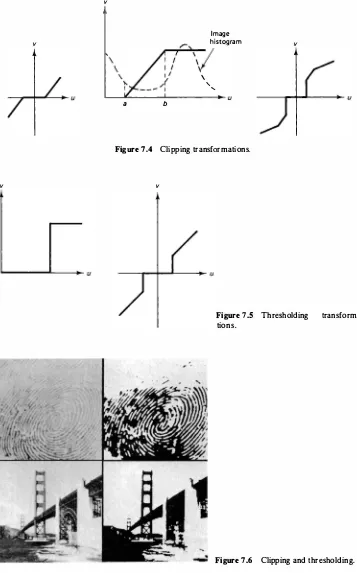
Clipping and Thresholding

A special case of contrast stretching where a = "Y = 0 (Fig. 7.4) is called clipping. This is useful for noise reduction when the input signal is known to lie in the range

(a, b].

Thresholding is a special case of clipping where a = b � t and the output becomes binary (Fig. 7.5). For example, a seemingly binary image, such as a printed page, does not give binary output when scanned because of sensor noise and back­ ground illumination variations. Thresholding is used to make such an image binary. Figure 7.6 shows examples of clipping and thresholding on images.

v

Sec. 7.2 Point Operations

Figure 7.2 Contrast stretching transfor­ mation. For dark region stretch a > 1, a = L/3; midregion stretch, 13 > 1, b = � L ; bright region stretch -y > 1 .

" " " " " "

Figure 7.3 Contrast stretching.

v

v

v

a b

Image histogram

\ ' _'

v

Figure 7 .4 Clipping transformations.

v

Figure 7.5 Thresholding transforma-tions.

Figure 7.6 Clipping and thresholding.

v

Digital Negative

Figure 7.7 Digital negative transforma­ tion.

A negative image can be obtained by reverse scaling of the gray levels according to the transformation (Fig. 7. 7)

v

=L

- u (7.3)

Figure 7.8 shows the digital negatives of different images. Digital negatives are useful in the display of medical images and in producing negative prints of images.

Intensity Level Slicing (Fig. 7.9)

Without background: v

= {L'

_0,

With background: v

={L,

_{u ,}

a :::;u :::;b otherwise a :::;u :::;b

otherwise

(7.4)

(7.5)

These transformations permit segmentation of certain gray level regions from the rest of the image. This technique is useful when different features of an image are contained in different gray levels. Figure 7.10 shows the result of intensity window slicing for segmentation of low-temperature regions (clouds, hurricane) of two images where high-intensity gray levels are proportional to low temperatures.

(a)

v

v

L

a b a b L

(a) Without background (b) With background

Figure 7.9 Intensity level slicing.

Bit Extraction

Suppose each image pixel is uniformly quantized to B bits. It is desired to extract the nth most-significant bit and display it. Let

Then we want the output to be

v =

{L,

_0,

It is easy to show that

Sec. 7.2 Point Operations

if kn = 1

otherwise (7.7)

(7.8)

Figure 7. IO Level slicing of intensity window [175, 250] . Top row: visual and infrared (IR) images; bottom row: seg­ mented images.

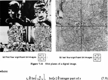
(a) First four significant bit images

�

; (b) last four significant bit images

�

Figure 7.11 8-bit planes of a digital image.

where

in � Int

[

_n

]

, Int[x] �integer part of x (7 .9)

Figure 7 . 1 1 _{shows the first 8 most-significant bit images of an 8-bit image. This}

transformation is useful in determining the number of visually significant bits in an image. In Fig. 7 . 1 1 _{only the first 6 bits are visually significant, because the}

remaining bits do not convey any information about the image structure.

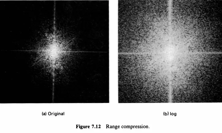
Range Compression

Sometimes the dynamic range of the image data may be very large. For example, the dynamic range of a typical unitarily transformed image is so large that only a few pixels are visible. The dynamic range can be compressed via the logarithmic transformation

v = c log1o(l + i u l) (7 . 10) where c is a scaling constant. This transformation enhances the small magnitude

pixels compared to those pixels with large magnitudes (Fig. 7 .1

2

)_.

Image Subtraction and Change Detection

(a) Original (bl log

Figure 7 .12 Range compression .

in a body. The blood stream is injected with a radio-opaque dye and X-ray images are taken before and after the injection. The difference of the two images yields a clear display of the blood-flow paths (see Fig. 9.44). Other applications of change detection are in security monitoring systems, automated inspection of printed circuits, and so on.

7.3 HISTOGRAM MODELING

The histogram of an image represents the relative frequency of occurrence of the various gray levels in the image. Histogram-modeling techniques modify an image so that its histogram has a desired shape. This is useful in stretching the low-contrast levels of images with narrow histograms. Histogram modeling has been found to be a powerful technique for image enhancement.

Histogram Equalization

In histogram equalization, the goal is to obtain a uniform histogram for the output image. Consider an image pixel value u 2: 0 to be a random variable with a continu­

ous probability density function

Pu

(a) and cumulative probability distribution F.. (a) � P[u ::5 u]. Then the random variable

Li Li

Ju

V ₌ F.. (u) =

0

Pu

(11) d11 (7. 1 1)

will be uniformly distributed over (0, 1) (Problem 7.3). To implement this transfor­ mation on digital images, suppose the input u has L _{gray levels} X;, i = 0, 1 , ... ,

L _-1 with probabilities

Pu

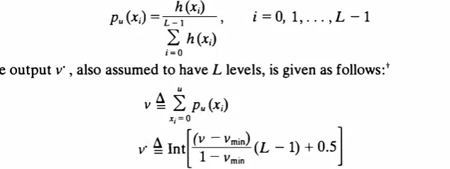
(x;). These probabilities can be determined from the

Uniform quantization

Figure 7.13 Histogram equalization transformation.

histogram of the image that gives h (x;), the number of pixels with gray level value x;.

Then

uniformly distributed only approximately because v _{is not a uniformly distributed}

variable (Problem 7.3). Figure 7.13 shows the histogram-equalization algorithm for digital images. From (7 . 13a) note that v is a discrete variable that takes the value

(7. 14)

i = O

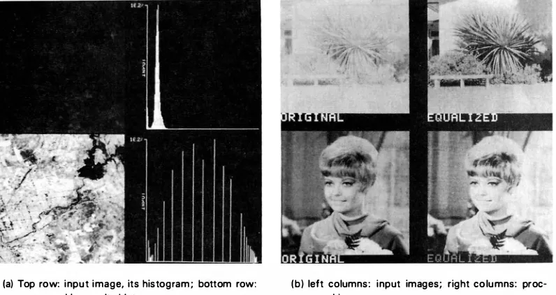
if u = xk. Equation (7.13b) simply uniformly requantizes the set {vk} to {vk}. Note that this requantization step is necessary because the probabilities Pu (xk) and Pv ( vk) are the same. Figure 7.14 shows some results of histogram equalization.

Histogram Modification

A generalization of the procedure of Fig. 7.13 is given in Fig. 7.15. The input gray level u is first transformed nonlinearly by f(u), and the output is uniformly quan­ tized. In histogram equalization, the function

u

f(u) =

L

Pu (x;) (7. 15)

x; = O

typically performs a compression of the input variable. Other choices of f(u) that have similar behavior are

n = 2, 3, . . . (7.16)

(a) Top row: input image, its histogram ; bottom row: processed image, its histogram;

(b) left columns: input images; right columns: proc­ essed images.

Figure 7.14 Histogram equalization.

f(u) = log (1 + u),

f(u) = ul'",

u � o

u � o, n = 2, 3, . . .

(7 . 17)

(7. 18)

These functions are similar to the companding transformations used in image quantization.

Histogram Specification

Suppose the random variable u � 0 _{with probability density Pu} (11) is to be trans­

formed to

v �

0 such that it has a specified probability density Pv (tr). For this to be

true, we define a uniform random variable

(7 . 19)

that also satisfies the relation

w =

r

Pv (y) dy = F;, (v)

0 (7.20)

Eliminating w, we obtain

Sec. 7.3 Histogra m Model ing

v

= F;1(F,, (u))

Uniform quantization

(7.21)

Figure 7.15 Histogram modification.

w w · ₌

Wn v· = _Yn

m�n:

{;;

n -w _;::: 0

}

_{F;, ( . )}

Figure 7.16 Histogram specification.

If u and

v

are given as discrete random variables that take values

xi

and _{Yi ,}

i

= 0, .. . , L -1 , with probabilities Pu

(xi)

and Pv

(yi),

respectively, then (7 .21) can be implemented approximately as follows. Define

u k

how this mapping is developed.

Pu (xi) - w·

Many image enhancement techniques are based on spatial operations performed on local neighborhoods of input pixels. Often, the image is convolved with a finite impulse response filter called

spatial mask.

Spatial Averaging and Spatial Low-pass Filtering

Here each pixel is replaced by a weighted average of its neighborhood pixels, that is,

v(m, n) = LL a(k, l)y(m -k, n -l)

_(k.l)<W

(7.23) where

y(m, n)

and

v(m, n)

are the input and output images, respectively, W is a suitably chosen window, and

a (k, l)

are the filter weights. A common class of spatial averaging filters has all equal weights, giving

LL y(m -k,n -l)

w(k.l)<W

(7.24)

, _ , _

Figure 7.17 Spatial averaging masks a (k, I).

v(m,

n)

=Hy(m,

n) +

i{y(m

- 1, n) +

y(m

+ l , n)

+

y(m,

_{n - 1)} +

y(m,

n + 1)}] (7 .25)

that is, each pixel is replaced by its average with the average of its nearest four pixels. Figure 7.17 shows some spatial averaging masks.

Spatial averaging is used for noise smoothing, low-pass filtering, and sub­ sampling of images. Suppose the observed image is given as

y(m,

n)

= u(m,

n) +

TJ(m,

n) (7.26) by a factor equal to the number of pixels in the window W. If the noiseless image

u(m,

n) is constant over the window W, then spatial averaging results in an im­

provement in the output signal-to-noise ratio by a factor of Nw. In practice the size of the window W is limited due to the fact that

u (m,

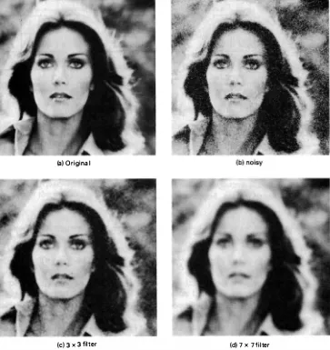
n) is not really constant, so that spatial averaging introduces a distortion in the form of blurring. Figure 7 .18 shows examples of spatial averaging of an image containing Gaussian noise.

Directional Smoothing

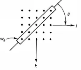
To protect the edges from blurring while smoothing, a directional averaging filter can be useful. Spatial averages

v (m,

n : 0) are calculated in several directions (see

gives the desired result. Figure 7.20 shows an example of this method.

(a) Original

(c) 3 x 3 filter (d) 7 x 7 filter

Figure 7.18 Spatial averaging filters for smoothing images containing Gaussian noise.

Median Filtering

Here the input pixel is replaced by the median of the pixels contained in a window around the pixel, that is,

v(m,

n

)

=

median{y(m -k,

n

-l), (k, l) � W} (7.30)

where W is a suitably chosen window. The algorithm for median filtering requires arranging the pixel values in the window in increasing or decreasing order and picking the middle value. Generally the window size is chosen so that Nw is odd. If

• •

.

. .

! . .

k Figure 7.19 Directional smoothing filter.

Typical windows are 3 x 3, 5 x 5, 7 x 7, or the five-point window considered for spatial averaging in Fig. 7. l 7c.

Example 7.2

Let {y (m)} = _{{2, 3, 8, 4, 2} and W = [ -1,} 0, 1]. The median filter output is given by

v(O)

�

2 (boundary value), v(l) = median {2, 3, 8} = 3 v (2) = median {3, 8, 4} = 4, v (3) = median {8, 4, 2} = 4 v(4) = 2 (boundary value)

Hence {v (m)} = {2, 3, 4, 4, 2}. If W contains an even number of pixels-for example, W = [-1, 0, 1 , 2]-then v(O) = 2, v(l) = 3, v(2) = median {2, 3, 8, 4} = (3 + 4)/2 = 3.5, and so on, gives {v(m)} = {2, 3, 3.5, 3.5, 2}.

The median filter has the following properties:

1. It is a nonlinear filter. Thus for two sequences x (m) and y (m) median{x (m) + y (m)} * median{x (m)} + median{y (m)}

(a) 5 x 5 spatial smoothing (b) directional smoothing Figure 7.20

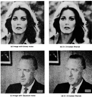
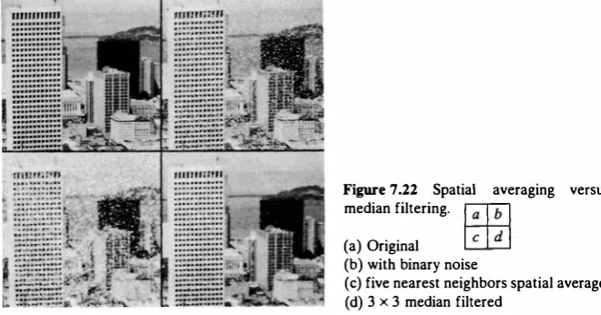
2. It is useful for removing isolated lines or pixels while preserving spatial resolu­ tions. Figure 7.21 shows that the median filter performs very well on images containing binary noise but performs poorly when the noise is Gaussian. Figure 7.22 compares median filtering with spatial averaging for images containing binary noise.

3. Its performance is poor when the number of noise pixels in the window is greater than or half the number of pixels in the window.

Since the median is the (Nw + 1)/2 largest value (Nw = odd), its search requires

(Nw -1) + (Nw -2) + · · · + (Nw - 1)/2 = 3(N2w - 1)/8 comparisons. This number

equals 30 for 3 x 3 windows and 224 for 5 x 5 windows. Using a more efficient

(a) Image with binary noise (b) 3 x 3 median filtered

Figure 7 .22 Spatial averaging versus median filtering.

(a) Original

(b) with binary noise

( c) five nearest neighbors spatial average (d) 3 x 3 median filtered

search technique, the number of comparisons can be reduced to approximately ! Nw log2 Nw [5]. For moving window medians, the operation count can be reduced further. For example, if k pixels are deleted and k new pixels are added to a window, then the new median can be found in no more than k(Nw + 1) comparisons. A practical two-dimensional median filter is the separable median filter, which is obtained by successive one-dimensional median filtering of rows and columns.

Other Smoothing Techniques

An alternative to median filtering for removing binary or isolated noise is to find the

spatial average according to (7 .24) and replace the pixel at m, n by this average

whenever the noise is large, that is, the quantity Iv (m, n) -y (m, n )I is greater than

some prescribed threshold. For additive Gaussian noise, more sophisticated smoothing algorithms are possible. These algorithms utilize the statistical proper­ ties of the image and the noise fields. Adaptive algorithms that adjust the filter response according to local variations in the statistical properties of the data are also possible. In many cases the noise is multiplicative. Noise-smoothing algorithms for such images can also be designed. These and other algorithms are considered in

Chapter 8.

Unsharp Masking and Crispening

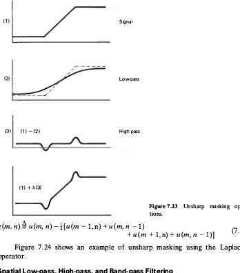
The unsharp masking technique is used commonly in the printing industry for crispening the edges. A signal proportional to the unsharp, or low-pass filtered, version of the image is subtracted from the image. This is equivalent to adding the gradient, or a high-pass signal, to the image (see Fig. 7 .23). In general the unsharp masking operation can be represented by

v (m, n) = u(m, n) + X.g(m, n) (7.31)

where X. > 0 and g (m, n) is a suitably defined gradient at (m, n ). A commonly used

gradient function is the discrete Laplacian

11 1

121

r

-_ __/

1 3)

(1 ) _-(2)

( 1 ) + ft.( 3)

Signal

Low-pass

High-pass

Figure 7.23 Unsharp masking opera­ tions.

g (m, n) � u (m, n) - Hu(m -1, n) + u(m, n - 1) _(7.32)

+ u(m + 1 , n) + u(m, n - 1)]

Figure 7.24 shows an example of unsharp masking using the Laplacian operator.

Spatial Low-pass, High-pass, and Band-pass Filtering

Earlier it was mentioned that a spatial averaging operation is a low-pass filter (Fig. 7.25a). If hLP(m, n) denotes a FIR low-pass filter, then a FIR high-pass filter,

hHP (m, n), can be defined as

hHP (m, n) = B(m, n) - hLP (m, n) (7.33)

Such a filter can be implemented by simply subtracting the low-pass filter output from its input (Fig. 7.25b). Typically, the low-pass filter would perform a relatively long-term spatial average (for example, on a 5 x 5, 7 x 7, or larger window).

A spatial band-pass filter can be characterized as (Fig. 7.25c)

hBP(m, n)

=

_{hL1 (m, n) - hL2 (m, n)} (7.34)

Figure 7.24 Unsharp masking. Original (left), enhanced (right).

u(m, n) Spatial averaging

(a) Spatial low-pass filter

u ( m, n) _LPF

u(m, n)

(b) Spatial high-pass filter

hL, ( m, n)

(c) Spatial band-pass fi lter

Figure 7 .25 Spatial filters.

Low-pass filters are useful for noise smoothing and interpolation. High-pass filters are useful in extracting edges and in sharpening images. Band-pass filters are useful in the enhancement of edges and other high-pass image characteristics in the presence of noise. Figure 7.26 shows examples of high-pass, low-pass and band-pass filters.

(e) (f) Figure 7.26 Spatial filtering examples.

Top row: original, high-pass, low-pass and band-pass filtered images. Bottom row: original and high-pass filtered images.

Inverse Contrast Ratio Mapping and Statistical Scaling

The ability of our visual system to detect an object in a uniform background depends on its size (resolution) and the contrast ratio, "f, which is defined as

a

'Y = ­µ (7.35)

where µ is the average luminance of the object and a is the standard deviation of the luminance of the object plus its surround. Now consider the inverse contrast ratio transformation

( ) _ µ(m, n)

v m, n - ( ) a m, n (7 .36)

where µ(m, n) and a(m, n) are the local mean and standard deviation of u (m, n) measured over a window W and are given by

µ(m, n) = N1

LL

u(m - k, n - l) w (k, l ) e W

{

1

}

112

a(m, n) =

_{N LL}

_{w (k, l ) e W} [u(m - k, n - l) - µ(m, n)]2

(7 .37a)

(7.37b)

This transformation generates an image where the weak (that is, low-contrast) edges are enhanced. A special case of this is the transformation

( ) _ u(m, n)

Figure 7.27 Inverse contrast ratio mapping of images. Faint edges in the originals have been enhanced. For example, note the bricks on the patio and suspension cables on the bridge.

which scales each pixel by its standard deviation to generate an image whose pixels have unity variance. This mapping is also called statistical scaling [13]. Figure 7.27 shows examples of inverse contrast ratio mapping.

Magnification and Interpolation (Zooming)

Often it is desired to zoom on a given region of an image. This requires taking an image and displaying it as a larger image.

Replication. _{Replication is a zero-order hold where each pixel along a scan}

line is repeated once and then each scan line is repeated. This is equivalent to taking an M x N image and interlacing it by rows and columns of zeros to obtain a

2M x 2N matrix and convolving the result with an array H, _{defined as}

H ₌

[� �]

(7.39)

This gives

v (m, n) = u(k, l), k

�

Int

[

�

J

, l =Int

[

�

J

, m, n = O, l, 2, . . . (7.40)

Figure 7.28 shows examples of interpolation by replication.

Linear Interpolation. Linear interpolation is a first order hold where a straight line is first fitted in between pixels along a row. Then pixels along each column are interpolated along a straight line. For example, for a 2 x 2 magnifica­ tion, linear interpolation along rows gives

Sec. 7.4

v1 (m, 2n) = u(m, n),

O s m s M - l, O s n s N - l v1 (m, 2n + 1) = Hu(m, n) + u(m, n + 1)],

O s m s M - l, O s n s N - l

Spatial Operations

(7.41)

0 3 0 2 0 3 3 2 2

[:

3 2 _Zero 0 0 0 0 0 0 _Convolve 3 3 2 2

5 6 interlace 4 0 5 0 6 0 4 4 5 5 6 6

0 0 0 0 0 0 4 4 5 5 6 6

(a)

(b)

Figure 7.28 Zooming by replication from 128 x 128 to 256 x 256 and 512 x 512 images.

Linear interpolation of the preceding along columns gives the first result as

v (2m, n) = v1 (m, n)

l

v (2m + 1, n) = Hv1 (m, n) + v1 (m + 1 , n)],

0 :s m :s M -1, 0 :s N :s 2N -1

(7.42)

Here it is assumed that the input image is zero outside [O, M - 1] x [O, N - 1]. The above result can also be obtained by convolving the 2M x 2N zero interlaced image with the array

1 0 7 0 Figure 7 .29 contains examples of linear interpolation. In most of the image process­ ing applications, linear interpolation performs quite satisfactorily. Higher-order (say, p) interpolation is possible by padding each row and each column of the input image by p rows and p columns of zeros, respectively, and convolving it p times with

H

(Fig. 7.30). For example p = 3 yields a cubic spline interpolation in between the pixels.

u(m, n) I nterlacing by p rows and

columns of zeros Convolve H

2

Figure 7.30 pth order interpolation.

Sec. 7.4 Spatial Operations

v(m, n)

p

7.5 TRANSFORM OPERATIONS

In the transform operation enhancement techniques, zero-memory operations are performed on a transformed image followed by the inverse transformation, as shown in Fig. 7.31. We start with the transformed image V = {v(k, /)} as

v = AUAT _(7.44)

where U = {u(m, n)} is the input image. Then the inverse transform of

v· (k, l) = f(v(k, l)) (7.45)

gives the enhanced image as

(7.46)

Generalized Linear Filtering

In generalized linear filtering, the zero-memory transform domain operation is a pixel-by-pixel multiplication

v· (k, l) = g (k, l)v (k, l) (7.47)

where g(k, l) is called a zonal mask. Figure 7.32 shows zonal masks for low-pass,

band-pass and high-pass filters for the OFT and other orthogonal transforms.

k

i

u(m, n)

0

Unitary v(k, / ) Point v· ( k, / ) Inverse u ' ( m, n)

transform operations transform

AUAT f( . ) A-1 _v· [AT ] -1

Figure 7.31 Image enhancement by transform filtering.

OCT

Hadamard Transform

OFT

Figure 7.33 Generalized linear filtering using DCT, and Hadamard transform and DFT. In each (a) original; (b) low-pass filtered; (c) band-pass filtered;

( d) high-pass filtered .

A filter of special interest is the inverse Gaussian filter, whose zonal mask for

N x N images is defined as

l

{

(k2 + 12)

}

g(k, I) = exp 2CT2 '

g(N - k, N - 1),

N 0 :5 k, I _{:5 2}

otherwise (7.48)

when A _{in (7.44) is the DFf. For other orthogonal transforms discussed in}

Chapter 5,

(k2 + 12)

g(k, I) = exp _{2CT2 ,} 0 :5 k, I :5 N - 1 (7.49)

This is a high-frequency emphasis filter that restores images blurred by atmospheric turbulence or other phenomena that can be modeled by Gaussian PSFs.

Figures 7.33 and 7.34 show some examples of generalized linear filtering.

Root Filtering

The transform coefficients v (k, I) can be written as

v (k, I) = Iv (k, l)lei9(k, 1> (7.50)

In root filtering, the a-root of the magnitude component of v (k, I) is taken, while retaining the phase component, to yield

v· (k, l) = lv (k, !Wei9(k,t>, 0 :5 a :5 l (7.51)

For common images, since the magnitude of v (k, I) is relatively smaller at higher

Originals Enhanced

Inverse Gaussian filtering

Lowpass filtering for noise smoothing (a) Original

(b) noisy (c) DCT filter

(d) Hadamard transform filter

(a) Original; _(b) a = 0 (phase only); (c) a = 0.5; (d) a = 0.7.

Figure 7 .35 Root filtering

spatial frequencies, the effect of a-rooting is to enhance higher spatial frequencies (low amplitudes) relative to lower spatial frequencies (high amplitudes). Figure 7.35

shows the effect of these filters. (Also see Fig. 8.19.)

Generalized Cepstrum and Homomorphic Filtering

If the magnitude term in (7 .51) is replaced by the logarithm of Iv (k, l)I and we define

s (k, l) � [log Iv (k, l)l]ei0(k. ll, lv(k, l)I > 0 (7.52)

then the inverse transform of s(k, l), denoted by c(m, n), is called the generalized

cepstrum of the image (Fig. 7 .36). In practice a positive constant is added to Iv (k, l)I

to prevent the logarithm from going to negative infinity. The image c(m, n) is also

JC

r - - - ,

I I

I mage I 1 Cepstrum

u(m, n) I v(k, / ) s(k, / ) I c(m, n) [log I v(k, I) 1 l eiBlk, ll A-' s(Ar)-t

1

Sec. 7.5

I

I I

L - - - �

(a) Generalized cepstrum and the generalized homomorphic transform JC .

c(m, n) s(k, _I) v(k, _{I )} u( m, n)

( I s I l }

(b) I nverse homomorphic transform, JC _,

mask

(c) Generalized homomorphic linear filtering

Figure 7.36 Generalized cepstrum and homomorphic filtering.

cepstrum of the building image generalized cepstra (a) original (b) OFT

(c) OCT

(d) Hadamard transform

Figure 7.37 Generalized cepstra:

.. _, ... · .. .

.._�;;."" � � .. .

called the generalized homomorphic transform, 9t", of the image u(m, n). The generalized homomorphic linear filter performs zero-memory operations on the %-transform of the image followed by inverse 9(:.transform, as shown in Fig. 7 .36. Examples of cepstra are given in Fig. 7.37. The homomorphic transformation reduces the dynamic range of the image in the transform domain and increases it in the cepstral domain.

7.6 MULTISPECTRAL IMAGE ENHANCEMENT

In multispectral imaging there is a sequence of I images U; (m, n), i = 1, 2, .. . , I, where the number I is typically between 2 and 12. It is desired to combine these images to generate a single or a few display images that are representative of their features. There are three common methods of enhancing such images.

Intensity Ratios

Define the ratios

Li u; (m, n)

R;.i (m, n) =

( ) ,

ui m, n i=l=j (7.53)

where U; (m, n) represents the intensity and is assumed to be positive. This method

Log-Ratios

Taking the logarithm on both sides of (7.53), we get

L;,1 � log R;,1 = log u; (m, n) - log u1 (m, n) (7.54)

The log-ratio L;,1 gives a better display when the dynamic range of R;,1 is very large, which can occur if the spectral features at a spatial location are quite different.

Principal Components

For each (m, n) define the I x 1 vector

[

u1 (m, n

)]

u(m, n) =

u2(

�

, n)

u1 (m, n)

(7.55)

The I x I KL transform of u(m, n), denoted by <I>, is determined from the auto­ correlation matrix of the ensemble of vectors

{u;

(m, n), i = 1 , . . . , I}. The rows of <I>, which are eigenvectors of the autocorrelation matrix, are arranged in decreasing order of their associated eigenvalues. Then for any 10 -:::; I, the images v; (m, n ),

i = 1 , ... , 10 obtained from the KL transformed vector v(m, n) = <l>u(m, n)

are the first 10 principal components of the multispectral images.

Figure 7.38 contains examples of multispectral image enhancement.

Sec. 7.6

Originals (top), visual band: (bottom), l.R.

Log Ratios Principal Compounds

Figure 7.38 Multispectral image enhancement. The clouds and land have been separated.

M ultispectral Image Enhancement

(7 .56)

7.7 FALSE COLOR AND PSEUDOCOLOR

Since we can distinguish many more colors than gray levels, the perceptual dynamic range of a display can be effectively increased by coding complex information in color. False color implies mapping a color image into another color image to provide a more striking color contrast (which may not be natural) to attract the attention of the viewer.

Pseudocolor refers to mapping a set of images u; (m, n), i = 1, . . . , / into a

color image. Usually the mapping is determined such that different features of the data set can be distinguished by different colors. Thus a large data set can be presented comprehensively to the viewer.

v (m n) 1

Input

Feature v2 (m, n) Color

extraction coordinate Display I mages v3 (m, n) transformation

u;(m, n)

Figure 7.39 Pseudocolor image enhancement.

Figure 7 .39 shows the general procedure for determining pseudocolor mappings. The given input images are mapped into three feature images, which are then mapped into the three color primaries. Suppose it is desired to pseudocolor a monochrome image. Then we have to map the gray levels onto a suitably chosen curve in the color space. One way is to keep the saturation (S* ) constant and map the gray level values into brightness (W* ) and the local spatial averages of gray levels into hue (0*).

Other methods are possible, including a pseudorandom mapping of gray levels into R, G, B coordinates, as is done in some image display systems. The comet Halley image shown on the cover page of this text is an example of pseudocolor image enhancement. Different densities of the comet surface (which is ice) were mapped into different colors.

For image data sets where the number of images is greater than or equal to three, the data set can be reduced to three ratios, three log-ratios, or three principal components, which are then mapped into suitable colors.

In general, the pseudocolor mappings are nonunique, and extensive inter­ active trials may be required to determine an acceptable mapping for displaying a given set of data.

7.8 COLOR IMAGE ENHANCEMENT

Input image enhancement coordinate

transformation independently transformed into another set of color coordinates, where the image in each coordinate is enhanced by its own (monochrome) image enhancement algorithm, which could be chosen suitably from the foregoing set of algorithms. The enhanced image coordinates Ti , Ti , T3 are inverse transformed to R' , G" , B" for display. Since each image plane Ti, (m, n), k = 1, 2, 3, is enhanced independently, care has to be taken so that the enhanced coordinates T;, are within the color gamut of the R-G-B system. The choice of color coordinate system Ti, , k = 1, 2, 3, in which enhancement algorithms are implemented may be problem-dependent.

7.9 SUMMARY

In this chapter we have presented several image enhancement techniques accom­ panied by examples. Image enhancement techniques can be improved if the en­ hancement criterion can be stated precisely. Often such criteria are application­ dependent, and the final enhancement algorithm can only be obtained by trial and error. Modern digital image display systems offer a variety of control function switches, which allow the user to enhance interactively an image for display.

P R O B L E M S

7.1 (Enhancement of a low-contrast image) Take a 25¢ coin; scan and digitize it to obtain

a 512 x 512 image.

a. Enhance it by a suitable contrast stretching transformation and compare it with

histogram equalization.

b. Perform unsharp masking and spatial high-pass operations and contrast stretch the

results. Compare their performance as edge enhancement operators.

7.2 Using (7.6) and (7.9), prove the formula (7.8) for extracting the nth bit of a pixel. 7.3 a. Show that the random variable v defined via (7.11) satisfies the condition

Prob[v s o-] = Prob[u s r1 (u-)] = F(r1 (o-)) = o-, where 0 < o- < 1. This means v

is uniformly distributed over (0, 1).

b. On the other hand, show that the digital transformation of (7 . 12) gives Pv ( vk ) = Pu (xk), where vk is given by (7 .14).

7.4 Develop an algorithm for (a) an M x M median filter, and (b) an M x 1 separable

median filter that minimizes the number of operations required for filtering N x N

images, where N � M. Compare the operation counts for M = 3, 5, 7.

7.5* (Adaptive unsharp masking) A powerful method of sharpening images in the pres­ ence of low levels of noise (such as film grain noise) is via the following algorithm [15] . The high-pass filter following eight directional masks (H0 ):

0 0 0 algorithm on a scanned photograph and compare with nonadaptive unsharp masking.

I mage _Directional Vo

mask Ho Threshold 7J Enhanced image

Figure P7.S Adaptive unsharp masking.

7.6* (Filtering using phase) One of the limitations of the noise-smoothing linear filters is that their frequency response has zero phase. This means the phase distortions due to noise remain unaffected by these algorithms. To see the effect of phase, enhance a noisy image (with, for instance, SNR = 3 dB) by spatial averaging and transform processing such that the phase of the enhanced image is the same as that of the original image (see Fig. P7.6). Display u (m, n), u (m, n) and u (m, n) and compare results at different noise levels. If, instead of preserving ll(k, l ), suppose we preserve 10% of the samples

"1(m, n)

�

[IDFf{exp j8(k, /)}] that have the largest magnitudes. Develop an algorithm for enhancing the noisy image now.

eiB(k,/l

Measure phase

u(m, n) u(m, n)

Noise smoothing

Noise 11(m, n)

7.7 Take a 512 x 512 image containing noise. Design low-pass, band-pass, and high-pass zonal masks in different transform domains such that their passbands contain equal

energy. Map the three filtered images into R, _G, B color components at each pixel and

display the resultant pseudocolor image.

7.8 Scan and digitize a low-contrast image (such as fingerprints or a coin). Develop a

technique based on contrast ratio mapping to bring out the faint edges in such images.

B I B L I O G R A P H Y

Section 7.1

General references on image enhancement include the several books on digital image processing cited in Chapter 1. Other surveys are given in:

1. H. C. Andrews. Computer Techniques in Image Processing. New York: Academic Press,

1970.

2. H. C. Andrews, A. G. Tescher and R. P. Kruger. "Image Processing by Digital

Computers." IEEE Spectrum 9 (1972): 20-32.

3. T. S. Huang. "Image Enhancement: A Review." Opto-Electronics 1 (1969): 49-59.

4. T. S. Huang, W. F. Schreiber and 0. J. Tretiak. "Image Processing." Proc. IEEE

59 (1971): 1586-1609.

5. J. S. Lim. "Image Enhancement." In Digital Image Processing Techniques (M. P.

Ekstrom, ed.) Chapter 1, pp. 1-51 . New York: Academic Press, 1984.

6. T. S. Huang (ed.). Two-Dimensional Digital Signal Processing I and II. Topics in Applied Physics, vols. 42-43. Berlin: Springer Verlag, 1981.

Sections 7.2 and 7.3

For gray level and histogram modification techniques:

7. R. Nathan. "Picture Enhancement for the Moon, Mars, and Man" in Pictorial Pattern

Recognition (G. C. Cheng, ed.). Washington, D.C. : Thompson, pp. 239-266, 1968.

8. F. Billingsley. "Applications of Digital Image Processing." Appl. Opt. 9 (February

1970): 289-299.

9. D. A. O'Handley and W. B. Green. "Recent Developments in Digital Image Processing

at the Image Processing Laboratory at the Jet Propulsion Laboratory." Proc. IEEE

60 (1972): 821-828.

10. R. E. Woods and R. C. Gonzalez. "Real Time Digital Image Enhancement," Proc. IEEE 69 (1981): 643-654.

Section 7.4

Further results on median filtering and other spatial neighborhood processing tech­ niques can be found in:

1 1 . J. W. Tukey. Exploratory Data Analysis. Reading, Mass. : Addison Wesley, 1971.

12. T. S. Huang and G. Y. Tang. "A Fast Two-Dimensional Median Filtering Algorithm."

IEEE Trans. Accoust. Speech, Signal Process. ASSP-27 (1979): 13-18.

13. R. H. Wallis. "An Approach for the Space Variant Restoration and Enhancement of

Images. " Proc. Symp. Current Math. Problems in Image Sci. (1976).

14. W. F. Schreiber. "Image Processing for Qulllity Improvement." Proc. IEEE, 66 (1978):

1640-1651 .

15. P. G . Powell and B. E . Bayer. " A Method for the Digital Enhancement of Unsharp,

Grainy Photographic Images." Proc. Int. Conf. Electronic Image Proc. , IEEE, U.K.

(July 1982): 179-183.

Section 7.5

For cepstral and homomorphic filtering based approaches see [4, 5] and:

16. T. G. Stockham, Jr. "Image Processing in the Context of a Visual Model." Proc. IEEE

60 (1972): 828-842.

Sections 7.6-7.8

For multispectral and pseudocolor enhancement techniques:

17. L. W. Nichols and J. Lamar. "Conversion of Infrared Images to Visible in Color."

Appl. Opt. 7 (September 1968): 1757.

18. E. R. Kreins and L. J. Allison. "Color Enhancement of Nimbus High Resolution

Infrared Radiometer Data." Appl. Opt. 9 (March 1970): 681 .