Selling, general and administration costs are the main components in the Income Statement. A large number of permanent staff in sales and marketing department will make the company dominated by the fixed costs. This fact could lead to sticky cost behavior. In addition, role of the manager can also cause the cost stickiness. When the company’s revenue decreases, manager may delay to decrease the cost or not even decrease cost at all. The objective of the study is to determine whether cost stickiness of selling, general and administrative in the Indonesian listed companies. This study applied log-linear data panel regression with 3605 firm years that is listed in Indonesian Stock Exchange (BEI) from 1993 – 2013. This study finds that selling, general, and administrative costs are sticky only for the manufacturing companies. Furthermore, the results show that adjustment of sales, general, and administrative costs delayed by the manager when revenue decreases, yet the cost stickiness will be reduced in the next period.
© 2014 IRJBS, All rights reserved. Keywords:
sticky cost,antisticky, selling,general, administrative costs, traditional cost model, alternative cost model.
Corresponding author: [email protected]
Benny Armanto, Karoline Melanika Tiono, Henry Suthiono
STIE Prasetiya Mulya, Jakarta
A R T I C L E I N F O A B S T R A C T
INTRODUCTION
Fluctuate costs are reaction from the shift in selling activities. The relation between cost with the activity can be explained by the traditional cost model. This model directly relates the cost with the activity in the company in a period. If the selling activity increases by ten percent, the cost will also increase by ten percent and vice versa. By the time, we can observe that increase in selling
activities will result greater increase in costs than by the time when selling activities decrease even in a proportional way.The phenomenon where costs swiftly increase when activities rise than the decrease when activities fall even in the same proportion and caused the costs to move asymmetrically are known as cost stickiness (Anderson et al., 2003).
Vol. 7 | No. 1 ISSN: 2089-6271
One of the components in selling, general and administrative costs (SGA costs) are salary for the permanent staff in sales and marketing. A nature of this cost is fixed cost. While the cost of commision for the sales and marketing are only variable costs. The more permanent staff in sales and marketing, will directly increase the fixed cost and create sticky cost behavior.
Costs that are sticky or less sticky, not just influenced by the proportion between fixed and variable cost, yet can also be influenced by the decision that are made by the managers (Anderson et al., 2003). As example, when the selling activities decrease, manager doesn’t directly reduce the human resources as he or she assumes that low sales will only be temporary. This decision causes sticky cost behavior and eventually bring alternative view from traditional cost model (Anderson et al., 2003). In this alternative view, cost incurred by the company is in relation with the manager’s decision due to allocation of companys’ resources and change in activities (Banker and Byzalov, 2013).
Insight or manager’s expectation regarding the company’s activity in the future, will influence the decision that will be taken. According to Banker et al. (2014), optimism and pesimism by a manager must be based on the demand condition in a period, where it will influence the decision of the manager.Then, Banker and Byzalov (2013) stated a manager who is confidence with the demand condition in the future will give weak response towards costs, delay to decrease the costs even when the sales falls and on the other hand will give strong response to the costs when there are increases in profit. While a pesimist manager toward the future demand will rapidly cut the cost when sales seems slowing down and will give slow response when there are increase in profit. This is called antisticky.
Asymmetry reaction from cost can also be caused by the agency problem (Banker and Byzalov, 2013). High level of cost stickiness may occur due
to the opportunity to use the company’s resources lavishly. This problem can be reduced with the practice of good corporate governance, where a manager can not invest excessively (Chen et al., 2012). On the other hand, although the agent factor can lead to cost stickiness, the agen factor could also lead to less cost stickiness. As an example when a manager gets incentives to reach target in a certain period, the manager quickly tackle the unused company’s resources caused by decreasing in revenue and hold to add new resources when revenue increases (Kama and Weiss, 2013).
Preliminary Research
Research on cost stickiness are using SGA Costs as the proxy to determine sticky cost behavior that occured by the company. SGA costs are used with few considerations: 1) Cost Stickiness are mostly found in SGA costs than in the category of other operational cost (Anderson et al., 2007), 2) SGA costs to be carefully calculated by the analyst and investor (Healy et al., 2000) and 3) SGA costs have a strong relation with the change in revenue, where many components from SGA costs influenced by the level of company’s revenue (Cooper and Kaplan, 1999 : 341)
A research done by Anderson, Banker and Janakiraman (2003) found that SGA costs will promptly increase when the activity rises and slowly decrease when the activity falls, where every increase of one percent in revenue, caused SGA costs increase by 0,55 percent, while decrease of one percent in revenue, only caused SGA costs to drop by 0,35%. Based on this finding, Anderson
et al., (2003) with the sample of public company in USA from 1979 – 1998 make a conclusion that SGA costsare behaving sticky.
variable that are applied in certain industry (Ely, 1991). As an example, West (2003) who done the research in 6 health center for 120 months, found that cost could behaving sticky when the manager’s control low. The same thing found by Balakrishnan and Gruca (2008) when researching a hospital in Ontario, cost behaving sticky when it is related with the main activity in the hospital, likecost that happened in the clinic of the hospital. It happened because it is not easy to reduce the cost (due to the low number of patients) and can badly affect to the low quality of treatments the patients receive.
The next thing that could influence the stickiness level of SGA costs are different characteristic from each country as the result of difference in industry structure, company’s characteristic and human resources market characteristic (Calleja et al., 2006). Calleja et al., (2006) who did the research in the companies through USA, UK, France and Germany, found that cost could behaving sticky (average increase 0,97 percent and decrease 0,91 percent for every one percent increase or decrease in revenue), yet for the company in France and Germany have more sticky behavior as the impact of the regulations. Moreover, Porporato and Werbin (2010) who did the research with sample from the banks in Argentina, Brazil and Canada from period of 2004-2009, found that cost behaving sticky with different percentage in each country.In Argentina, Brazil and Canada there were increases in each country as 0,60 percent, 0,82 percent and 0,94 percent as well decreases as 0,38 percent, 0,48 percent and 0,55 percent for every increases/ decreases one percent of revenue.
Some research related with cost stickiness have been done in Indonesia with specific sample. Research with the sample from the Indonesian State Owned Enterprises (BUMN) didn’t show the phenomenon of sticky cost, however the highest the intensity of the company’s asset, would cause bigger sticky behavior (Rahmadi, 2012). Other research used the sample from Bank Perkreditan
Rakyat (BPR) located in Jawa Tengah, also did not find the phenomenon of cost stickiness, yet the result were showing that the ownership by government to the BPR in regency area has the higher level of stickiness compare to the BPR managed by provincial government. This could happen since the BPR in regency area are in low position compare to the BPR managed by provincial government that it is easier for intervention by the local government which cause the cost stickiness (Erlyna, 2013).Further on, in manufacturing companies were found the contradictory result. Research with the sample from 2007-2009 found the phenomenon of cost stickiness in the Indonesian manufacturing companies, however the intensity of the asset was not significant to the stickiness of cost (Kusu, 2012). On the contrary, research with the companies sample from 2009-2011, didn’t find cost stickiness in the Indonesian manufacturing companies, yet found that the higher the intensity of companies asset, would likely cause the higher level of stickiness (Endarwati, 2013).
Research on cost stickiness of the companies in Indonesia were showing inconsistent result. Yet seing the trends of the research in Indonesia that is not sticky, the proposed hypothesis as shown below:
H1= Proportion of increase in SGA costs when revenueis up will be smaller from or same with the decrease in SGA costs when revenue is down.
Cost Stickiness Between the Sector
In Indonesia, companies could be categorize into three main sectors (Buku Panduan Indeks Harga Saham Bursa Efek Indonesia 2010). The main sector consist of primary sector (extractive industry), secondary sector (manufacture industry) and tertiary sector (service industry). Each of the three main industry then describe into nine sector industry then categorize into 56 sub-sector.
marketing.While, the main account in SGA costs that is easily to adjust with increase or decrease in sales, such as salary for temporary staff/contract/ depends on commision, training expense, advertising expense, and administration expense.
Primarysector (extractive industry) consists of agriculture and mining sector. SGA costs in these sectors are usually small because the company’s relation, that is busines to business,only require small staff in sales and marketing. So, the SGA costs for the primary sector are usually behaving less sticky.
The secondary sector (manufacture industry) consists of basic industry and chemicals, miscellaneous industry and consumer goods industry. The trend of the company’s relation in this sector are business to business that require many employees in sales and marketing department, so the SGA costs for the secondary sector is usually behaving sticky.
The tertiary sector (service industry) consists of property, real estate, and building construction industry, infrastructure, utilities and transportation industry, and trade, services, and investment industry.The trend of the company’s relation in this sector are business to customer that doesn’t require many permanent staff in sales and marketing department. Staff in these sectors are usually part timer or freelance or based on comission depend on the number of sales, so the SGA costs in these sectors are usually behaving less sticky.
Based on the statement above, the proposed hypothesis as shown below:
H2= SGA costs in extractive industry and service industry are behaving less sticky, while manufacture industry tend to behaving sticky.
Not only manager’s optimism that delay the decrease of the unnecessary cost, yet the
adjustment costs are another factor that neededto be taken care when the revenue decrease. Adjustment costsare cost that can be material or psychological that are spent by the company to respond the adjusment in company’s activity (Balakrishnan and Gruca, 2008). For example, to terminate a staff, terminate the contract, and to stop the operation. Decision to adjust the cost, for the sake of unused resources, will become more expensive to the company if the situation or activities of the company back to normal and termination has been done, in this case new resources has to be re-hire again. This fact make the manager to be in a difficult position to terminate the contract with the outsource provider, to decrease the resources are not as interesting as to increase the resources with the same proportion (Cooper and Haltiwanger, 2006).Banker and Byzalov (2013) stated that manager will choose to hold the unuseful resources when the revenue decrease, than to release the resources with some cost adjustment.Based on the statement above, manager will opt to hold the resources and wait for the certainty and look for the information that the company’s revenue will decrease for the long term.The manager put into consideration which opt will give the cheapest cost with positive effect in the long term. Other information that should be considered by the manager is the amount of the adjustment cost that needs to be settled in the next period, if the manager opts to hold the resources or even add new resources in this period (Banker and Byzalov, 2013).
of cost reducing, thus becoming as a factor of the sticky cost (Sorros and Karagiorgos, 2013).
Moreover, the decision to spend the adjustment cost to decrease the unuseful resources can not be done directly. As example, to terminate the contract with third party, it takes a long timeand have to pay fines at the end. The delay in making decision by managers and the lag time required when the decision was taken until realized, will result in sticky behavior of the SGA costs in the period, but will disappear or be reduced in the next period.
Based on the description, proposed the following hypothesis:
H3 = Stickiness of SGA costs will remain or increase in the next period.
METHODS
Types and Research Variable
This research includes in the study of causal and will use three variables: 1) the cost, which is proxied by the cost of sales, general, and administrative (SGA costs), 2) the revenue, which is proxied by the value of revenue, and 3) a dummy variable, variables are used to differentiate between the period of observation.
Variable of costs are dependent due to it fluctuates with revenue in certain period. Dummy variables are a differentiate variable with constant value between one and zero. One is given when the revenue in period t-1 higher than revenue in t
period and vice versa.
Population and Sample
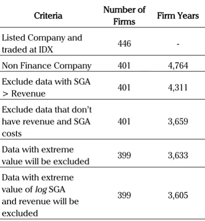
The study used a population of all public companies in Indonesia, listed in Indonesian Stock Exchange for 21 years range 1993-2013. Data were collected from the database of Capital IQ (Compustat) and forthe data are not available, searched again on the Indonesian Stock Exchange. Samples were then selected using the following criteria:
Data from the year 1993-2013 is used for the reason that the research can provide a broad overview and fundamental to the sticky behavior in the Indonesian company from the beginning of the data availability. Empty or missing data from 1998 due to financial crisis that occurred in Indonesia. The data that were empty, sought in other databases such as Indonesian Capital Market Directory (ICMD). If the data is not found then the observation data in years t-n, t and t + 1
in the company will be excluded from the sample.
The study will use panel data with unbalanced type because each company in the sample had a span of different operational year. The financial statements were obtained varied from 3 to 21 years old depending on the company’s founding. Although the use of panel data with the balanced type are better than unbalanced, however the study did not seek to exclude the observation that exist to produce a balanced panel data. This is done so the bias selection does not occur in the research.
Following Anderson et al. (2003), companies which has a larger SGA costs than revenue are excluded from the sample. Larger SGA costs
Criteria Number of Firms Firm Years
Listed Company and
traded at IDX 446
-Non Finance Company 401 4,764
Exclude data with SGA
> Revenue 401 4,311
Exclude data that don’t have revenue and SGA costs
401 3,659
Data with extreme
value will be excluded 399 3,633
Data with extreme value of log SGA and revenue will be excluded
399 3,605
from revenue will indicate a negative value in the Income Statement and not suitable for the research model.
Analysis Method
The study use log-linear panel data regression to measure the cost stickiness. One of the research model that will be used is among the following (Greene, 2012: 285-287): 1) constant coefficients or pooled-regression model, 2) fixed-effect model, and 3) random effects model. Some tests will be done before determining the model to be used in research. Several tests will be conducted to determine the models are: 1) Chow test, 2) Breusch-Pagan LM test, and 3) Hausman test.
The first model, made by Anderson, Banker, and Janakiraman (2003), arranged to test the first hypothesis, the increase in SGA costs as revenueriseswill be greater than the decrease in SGA costs when revenuefalls. The hypothesis will be test with the following equation:
t
The first model is the examination base of the relationship between changes in revenue withstickiness of cost. Estimations of the model is cross-sectional with varied industries and difference in companies sizes, the format of the log and ratio will increase the comparisons accuracy of the variables between companies (Anderson
et al., 2003). In addition, the format of the ratio and log fromrevenue and SGA costs also aims to provide easy result to be compare and enables the economic interpretation of the coefficients obtained (Anderson et al., 2003). Then, Anderson
et al. (2003) describes that since decrease_ dummy value is zero when revenue increases, the coefficient β1 measures the percentage increase in
SGA costs when revenue increased by one percent. While decrease_dummy worth one when revenue decreases, the coefficient β1 + β2 measures the percentage increase in SGA costs when revenue fall by one percent. Furthermore, if SGA costs are sticky, the change in the SGA costs when revenue increases, will be greater than the changes when revenue decreases. Thus, the empirical hypothesis for stickiness, condition of β1 is greater than zero, is that zβ2 smaller than zero.
To test the second hypothesis, the SGA costs in the industry producing extractive and services industry will behave less sticky, while the manufacturing industry will behave sticky, we will usethe first model as abase for each industry.
The second model, also made by Anderson, Banker, and Janakiraman (2003), arrange to test the third hypothesis, stickiness of SGA costs will remain or increase in the next period. The third hypothesis will be tested with the following equation:
The second model is the extension of the first model that incorporate additional one period of revenue adjustment in relation to the time required by the manager. Acceptance condition of coefficient in second model isthe same as those in the first model with additional coefficients β3
to changes in revenue. Coefficient β4is positive and significant indicates a reduction in the level of stickiness of the SGA costs in the period after the decline in revenue occurred (β4<|β2|).
RESULTS AND DISCUSSION Descriptive Statistics
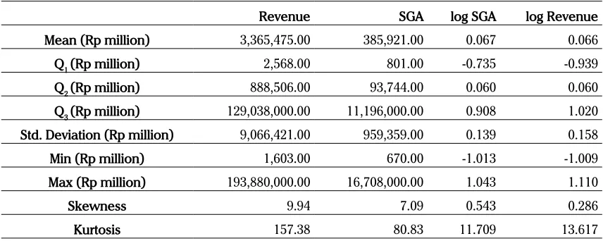
Table 2 below shows the average non-financial public company in Indonesia with revenue of 3,365,475 million rupiah and standarddeviationof 9,066,421 million rupiah. The revenue varies between 1,603 million to 193,880,000 million rupiah. Meanwhile, the average company in Indonesia has the SGA costs of 385,921 million rupiahwith standard deviation of 959,359 million rupiah. SGA costs vary from the smallest 670 million to 16,708,000million rupiah. Quartile data can be interpreted as follows. As much as 25 percent of the revenue in public company in Indonesia has a value less than or equal to 2,568 million rupiah. While 50 percent of the revenue data are in the range of 2,568 million rupiah and 129,038,000 million rupiah. For SGA costs, 25 percent of the data has a value less than or equal to 801 million rupiah. 50 percent of the SGA costs data were in the range of 801 million rupiah and 11,196,000 million rupiah.
Bigger standard deviation occurred because of large amount of data and taken from a variety of
industry. Every industry has a different cost and revenue structure. Bigger standard deviation are also caused by the variation of the companies size that involve in the research sample.
The data that have been normalized with log function does not show much different from the data that is not normalize. Skewness and kurtosis values of both types of data indicate the potential normality problem that occur at variable.
The conclusion that can be drawn from the descriptive statistics is that the Indonesian companies traded on Indonesian Stock Exchange (BEI) come from industries with varied size of firm. As a result of the diverse company size, it can be seen that the value of the revenue and SGA costs of each company is quite different one anotherand with large standard deviation. Companies with biggerrevenue and SGA costs were dominated by companies from the mining and manufacturing industries.
Furthermore, revenue and SGA costs of the companies that have been operating for at least one decade, would tend to have extreme movements in 1997, 1998 and 1999. It happened due to financial crisis in Indonesia. In 1997 to 1998, would seem an extreme decline of the value of revenue and SGA costs, on the other hand from
Revenue SGA log SGA log Revenue
Mean (Rp million) 3,365,475.00 385,921.00 0.067 0.066
Q1 (Rp million) 2,568.00 801.00 -0.735 -0.939
Q2 (Rp million) 888,506.00 93,744.00 0.060 0.060
Q3 (Rp million) 129,038,000.00 11,196,000.00 0.908 1.020
Std. Deviation (Rp million) 9,066,421.00 959,359.00 0.139 0.158
Min (Rp million) 1,603.00 670.00 -1.013 -1.009
Max (Rp million) 193,880,000.00 16,708,000.00 1.043 1.110
Skewness 9.94 7.09 0.543 0.286
Kurtosis 157.38 80.83 11.709 13.617
1998 to 1999 have a very extreme rise.For example, PT Benakat Integra (BIPI) which recorded an increase of 5,572 percent from 1998 to 1999 that should be excluded from the sample.
Classical Assumption Test and Regression Model Determination
The classical assumption result has been made that the research model will be Best Linear Unbias Estimator (BLUE), sothere is no relating problem to heteroscedasticity, autocorrelation and multicollinearity. To test for normality, there is a problem that one of the factor, can be caused by the spread of the data that is too large and the number of extreme data. However, according to Gujarati (2004: 110), this can be overcome by increasing the number of observations used. This study uses the 3605 observation of the 399 companies in the period of 1993 to 2013, so that the data distribution of the variables can be assumed to be normal.
After carrying out the chow test, Breusch Lagrange Multiplier test (LM), and Hausman test, the research model is suitable with the fixed effect (FE).
Effects of Changes in Revenue on the Stickiness of SGA costs
Results of regression test performed to see the effect of changes in revenue to the stickiness of SGA costs, can be seen in table 3, with the value of
Adjusted R2of 0.2821.
Coef (t-stat) p-value Logrev 0.424
(7.78)***
0.000
decrease_dummy -0.003 (-0.37)
0.709
constant 0.040 (6.89)***
0.000
Prob > F 0.000 *** Significant at the level 0.01 ** Significant at the level 0.05 * Significant at the level 0.10 Source: Data processing 2014 Table 3. Results of Hypothesis 1
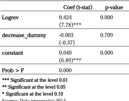
The first model was statistically significant as proved by the value of 0,000 in the F test that the revenue variable simultaneously affect the SGA costs. Coefficient value β1(logrev) of 0.424 andt
7.78 are significant, partially prove that revenue as independent variables affect the SGA costsas the dependent variable. β1 coefficient value indicates an increase in SGA costs of 0.424 percent for every one percent increase in revenue.
β2value (decrease_dummy) of -0.003 with a t
value of -0.37 is not significant, does not prove that revenue affects SGA costs. The value of the negative coefficient β2 provide a picture that is consistent with the sticky cost phenomenon. This is due to the value of β1 + β2 is 0.421 which indicates that the SGA costsdecreased by 0.421 percent for every one percent decline in revenue. This means SGA costs will go down slowly than the increase as revenue rise. This indicates the presence of sticky SGA costs phenomenon, the circumstances in which the cost will go down faster than the increase in the proportion of the increase and decrease inrevenue proportionately. However, because the tvalue which is not significant at β2, it can be concluded that the sticky behavior of SGA costs in Indonesian company can not be prove. This indicates thepotential antisticky behavior within the company in Indonesia, a condition where the cost come down faster than the increase for the same proportion of revenue changes.
Analysis on Industrial Sector
conditions of each country are very different when viewed in terms of external and internal. For example, the manufacturing industry in Indonesia is not necessarily indicate sticky behavior when compared with the United States. Therefore, in addition to the overall calculation of all samples in Indonesia, the calculation will also be divided into three main sectors according to the Stock Exchange (Buku Panduan Indeks Harga Saham Bursa Efek 2010), namely theextractive sector, manufacturing sector, and service sector.
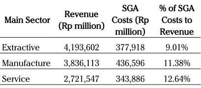
Table 4 shows that the extractive sector’s percentage of SGA costs to revenues is the smallest compared to the manufacturing sector and service sector, which amounted to 9.01 percent. This is due to the company’s relationship business to business and requires minimal sales and marketing staff, so the SGA costs of this sector behave less sticky. For the manufacturing sector where it is business to business relation, it takes a lot of staff remain as part of sales and marketing, resulting the percentage of SGA costs to revenue is higher than the extractive sector. While the service sector, the percentage of SGA costs to revenue is higher than most other sectors. This is due to the sector that needs a lot of sales and marketing staff, but most of them are part-time or commission basis. The result in the SGA costs for services sector are less sticky than the manufacturing sector.
Main Sector (Rp million)Revenue Costs (Rp SGA million)
% of SGA Costs to Revenue
Extractive 4,193,602 377,918 9.01%
Manufacture 3,836,113 436,596 11.38%
Service 2,721,547 343,886 12.64%
Source: Data processing 2014
Table 4. Revenue and SGA costs by the Main Sector
a) Analysis in theExtractive Industry
After do the panel test and classical assumption by using the data of 448 observations of 56 companies and the adjusted value R2 of 0.2945, there is a
normality problem and heteroscedasticity, means to sample the extractiveindustry is no longer BLUE. However, regression studies will be transformed into a model of Generalized Least Square (GLS). Further regression in extractiveindustry with the following results:
Coef (t-stat) p-value Logrev 0.428
(9.98)***
0.000
decrease_dummy -0.023 (-1.30)
0.193
constant 0.051 (5.06)***
0.000
Prob > chi2 0.000 *** Significant at the level 0.01 ** Significant at the level 0.05 * Significant at the level 0.10 Source: Data processing 2014 Table 5. Extractive Industry
We used the GLS modeland then choosed to using the chi test other than the F test. Result of chi test is 0.000 means that the model is statistically significant and revenue variables simultaneously affect the SGA costs. From Table 5 thevalue β1
(logrev) of 0.428 is positive and significant with a
t-value of 9.98. The value of β2 (decrease_dummy) is -0.023 with a t-value of -1.30, yet not significant, shows that therevenue does not affectthe SGA costs partially and the value of β1 + β2 is 0.405.
The coefficient value can be interpreted as an increase in SGA costs of 0.428 percent when revenue rise one percent and SGA costs will go down 0.405 percent when revenue fall one percent. Negative values of β2 indicates sticky cost behavior, yet from the results of the t test, the t
value was not significant, so it can be concluded that the sticky behavior of the SGA costs does not appear on the extractive industry in Indonesia.
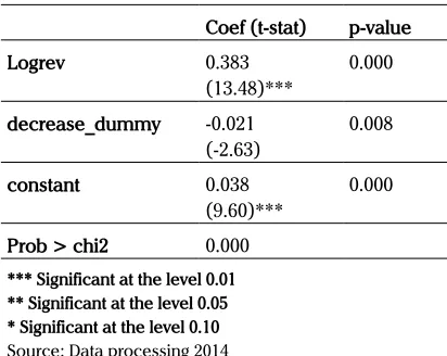
b) Analysis in the Manufacture Industry
companies and adjusted R2 value of 0.2065, there
was a normality problem and heteroscedasticity, that means the sample in the manufacture industry is no longer BLUE. However, regression studies will be transformed into a GLS model. Furthermore, the regression was done in the manufacture industry with the following results:
Coef (t-stat) p-value Logrev 0.383
(13.48)***
0.000
decrease_dummy -0.021 (-2.63)
0.008
constant 0.038 (9.60)***
0.000
Prob > chi2 0.000 *** Significant at the level 0.01 ** Significant at the level 0.05 * Significant at the level 0.10 Source: Data processing 2014 Table 6. Manufacture Industry
We used the GLS model and then choosed to using the chi test other than the F test. Result of chi test is 0.000 means that the model is statistically significant and revenue variables simultaneously affect the SGA costs. From Table 6 the value β1
(logrev) of 0.383 is positive and significant with a
t-value of 13.48. The value of β2 (decrease_dummy) is -0.021 with a significant t-value of -2.63, shows that the revenue affects the SGA costs partially and the value of β1 + β2 is 0.362.
The coefficient value can be interpreted as an increase in SGA costs of 0.383 percent when revenue rise one percent and SGA costs will go down 0.362 percent when revenue fall one percent. Each of these value has a significant
t-value, indicates the existence of sticky behavior in the SGA costs in Indonesian manufacture industry.
c) Analysis in the Service Industry
After do the panel test and classical assumption by using the data of 1,640 observations from 202 companies and adjusted R2 value of 0.31, there
was a normality problem, heteroskedasticity, and autocorrelation, that means the sample in the service industry is no longer BLUE. However, regression studies will be transformed into a GLS model. Furthermore, the regression was done in the service industry with the following results:
Coef (t-stat) p-value Logrev 0.486
(22.52)***
0.000
decrease_dummy 0.007 (0.75)
0.456
constant 0.039 (8.52)***
0.000
Prob > chi2 0.000 *** Significant at the level 0.01 ** Significant at the level 0.05 * Significant at the level 0.10 Source: Data processing 2014 Table 7. Service Industry
We used the GLS model and then choosed to using the chi test other than the F test. Result of chi test is 0.000 means that the model is statistically significant and revenue variables simultaneously affecting the SGA costs. From Table 7 the value
β1 (logrev) of 0.486 is positive and significant with a t-value of 22.52. The value of β2 is 0.007 with a
t-value of 0.75 which is not significant, shows that the revenue does not affectthe SGA costs partially and the value of β1 + β2 is 0.493.
The coefficient value can be interpreted as an increase in SGA costs of 0.486 percent when revenue rise one percent and SGA costs will go down 0.493 percent when revenue fall one percent. Value of β2 indicates a positive value, it is an indication of antisticky behavior toward SGA costs in service industry. Further analysis of the z
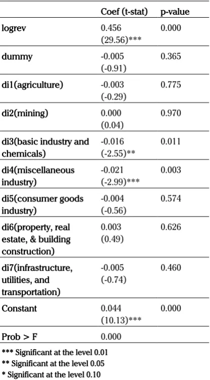
d) Analysis among Industries
Here are the results of the regression among industries. This is done to determine which industries have different results from the basic industries. Basic industries in the following regression are trade, service,and investment industry. Regression results using 3,605 observations with adjusted R2 value of 0.284 is as
follow:
di3(basic industry and chemicals) estate, & building construction) *** Significant at the level 0.01 ** Significant at the level 0.05 * Significant at the level 0.10 Source: Data processing 2014 Table 8. Among Industries
Table 8 present the calculation results of the regression among industries of eight industrial sectors in Indonesia. Result of the F test value on regression above 0.000,means the model is statistically significant and revenue simultaneously affects the SGA costs. Eight industrial sector in this research is part of the three main sectors.
Regression among industries are done to find out the difference in the stickiness level among industries to the basic industries. Industrial base has been set derived from trade, services, and investment.
The significant t-value were shown by the basic industry and chemicals and miscellaneous industry. Both the industrial sector has a significant t-value of -2.55 and -2.99. Basic industry and chemicalshas a significant coefficient of -0.016 compared to base industry, namely trade, services, and investment, so the basic industry and chemicals tends to be less sticky at -0.016 percent. The coefficient for miscellaneous industry of -0.021 percent, means when compared with base industry, the miscellaneous industry will tend to be less sticky at -0.021 percent. Other industries have a coefficient value and different t-value, but because its value is not statistically significant, it can be concluded that these industries are not much different from the base industry.
Regression result among industries are in line with the result shown in the regression by industry. In the regression by industry, manufacture industry shows the sticky cost behavior, while in extractive industry and service industry does not show such behavior. Basic industry and chemicals and miscellaneous industry are part of the manufacture industry. This is the factor that makes the coefficient valueof the two sectors have significant result.
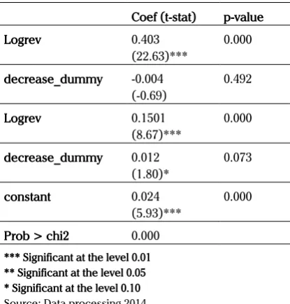
SGA Costs Stickiness for the Next Period
For the third hypothesis, testing is done with the second model. Stickiness of the SGA costs expected to decrease in the period after revenue is reduced. Regression results using data from 3,192 observations with adjusted R2 value of 0.28 is as
Table 9.
SGA costs. Furthermore, the lagged revenue and dummy variables are incorporate into the model and regression test to see the effects of delays in decision making of manager in SGA costs that expected to be reduced in the next period.
Results obtained on β1 and β2 in the second model is the value of β1 at 0.403 with a significant
t-value of 22.63 and β2 value of -0.004 with an insignificant t-value of -0.69. This means that the revenuevariable partially affect SGA costs only on β1. Similar to the result in the first model, the coefficients indicate a potential sticky behavior of the SGA costs. This is shown by the increase in cost of 0.403 percent over one percent increase in revenue and lower costs by 0.399 percent over one percent decline in revenue. However, the insignificantt-value of β2 conclude that although the coefficient is indicating the sticky cost, yet the insignificant value indicate the existence of sticky cost in Indonesian companies through the second model can not be proven. These results are similar to the first model. Thus, it can be concluded that there are indications of the antisticky behavior on the SGA costs in the second model.
To see the impact of the delay in the manager’s decision, then β3 and β4 are the coefficient to
consider.Positive and significant β3value of 0.1501 (t = 8.67) showed a delayed in the adjustment to the SGA costs when therevenue decline. Positive
β4 value of 0.012 indicates a reduction in SGA costs stickiness in the period after revenuedecreased. Significant β4 value with t-value of 1.80, means the stickiness of the cost turned to be decreased after a period of the decline in revenue.It can be concluded, eventhough the cost of stickiness in the Indonesian company can not be proved, the adjustment delay in the resources is still happen.
MANAGERIAL IMPLICATIONS
Shift in company’s revenue are quite common. Positive changes make the manager to add the resources in order for the smooth operations and company’s demand can be fulfilled, on the other hand when the shift is negative, the manager is expected to adjust the unuseful resources to do not be a burden to the company.
From the regression test results, it can be concluded that the sticky behavior of SGA costs in Indonesian companies can not be proven. This indicates a relatively good decision making by managers related to the allocation of company’s resources, such as pay the adjustment cost when revenue decline, or when revenue increase, manageralso consider the adjustment costs to be incurred in the next periods and only add resources until to the optimum level.
The absence of strong prove to support the sticky cost phenomenon in the Indonesian company is different with findings that had been concluded by the study of Anderson, Banker, and Janakiraman (2003). Generalization conducted by research in the United States in essence can not be done in each country. However, empirical prove in Indonesia shows that stickiness of SGA costs will be decreased in the period after revenue decline, which is consistent with the previous research.
CONCLUSION
The objective of this research is to analyze the
Coef (t-stat) p-value Logrev 0.403
(22.63)***
0.000
decrease_dummy -0.004 (-0.69)
0.492
Logrev 0.1501 (8.67)***
0.000
decrease_dummy 0.012 (1.80)*
0.073
constant 0.024 (5.93)***
0.000
behavior cost of sales, general, and administrative (SGA) in the Indonesian company. This research is done to capture the sticky behavior of the SGA costs toward the shift in revenue. Sticky cost behavior is an asymmetry reaction from the delay in cost decreasing than increasing for every shift in proportional revenue. In addition, the research is done to have the overview whether the manager delay to make decisions in regard to adjust the resources.
The research shows the results with an average increase in SGA costs in Indonesian company of 0.424 percent for every one percent increase in revenue and SGA costs will decrease by an average of 0.421 percent for every one percent decline in revenue. Although these results suggest the potential of sticky behavior of SGA costs, yet the value is not statistically significant. It can be concluded that the SGA costs in Indonesia indicate the antisticky behavior.
Furthermore, when the sample is divided into three main sectors, the stickiness of SGA costs was found in the manufacture industry, in every one percent increase in revenue, the SGA costs will increase by 0.383 percent and every one percent decrease in revenue, the SGA costs will decline by 0.362 percent. Whereas, for the extractive and service industry, the sticky behavior of SGA costs was not found.
In the second model, the results obtain indicate that the SGA costs increased by 0.403 percent for every one percent increase in revenue and will decreased by 0.399 percent for every one percent decline in revenue. However, in line with the results shown in the first model, these results were not statistically significant, it was concluded to be not proven. Furthermore, the test results indicate the presence of adjustment in SGA costs when delayed by the manager while the revenue decline and reduction in stickiness in the next period after the revenue decline.
Findings indication of the antisticky behavior of the SGA costs in Indonesian companies provide the different signals from the research that had been done previously. The differences can be due to many things, such as the manager’s behavior in making decisions. The antisticky behavior can occur because the manager in Indonesian companies are quite pessimistic, so when the revenue decrease, the manager would immediately reduce the resources or make some cost adjustment. In addition, Indonesia is a developing country, this has resulted in the fluctuations in revenue and cost a lot more difficult to predict than the developed countries. Whereas the previous research were using developed countries as the sample, it would be different when the research conducted in Indonesia.
R E F E R E N C E S
Bursa Efek Indonesia.(2010). Buku Panduan Indeks Harga Saham Bursa Efek Indonesia 2010.
Anderson, Mark C., Banker, R. D., & Janakiraman, S.N. (2003). «Are selling, general, and administrative costs “sticky”?.»Journal of Accounting Research 41.1.2003, 47-63.
Anderson, M., Banker, R., Huang, R., & Janakiraman, S. (2007). Cost behavior and fundamental analysis of SG&A costs. Journal of Accounting, Auditing & Finance, 22(1).2007: 1-28.
Balakrishnan, R. and Gruca, T. S. (2008). Cost stickiness and core competency : a note. Contemporary Accounting Research 25.4.2008: 993-1006.
Banker, R. D., & Byzalov, D. (2013). Asymmetric cost behavior. Tersedia di http://ssrn.com/abstract=2312779.
Calleja, K., Steliaros, M., & Thomas, D. C. (2006). A note on cost stickiness : some international comparisons. Management Accounting Research 17.2.2006 : 127-140.
Chen, C. X., Lu, H., & Sougiannis, T. (2012). The agency problem, corporate governance, and the asymmetrical behavior of selling, general, and administrative costs. Contemporary Accounting Research 29.1.2012 : 252-282.
Cooper, R. & Kaplan, R. S. (1999). The design of cost management systems : text and cases. Prentice Hall.
Cooper, R. W. and Haltiwanger, J.C. (2006). On the nature of capital adjustment costs. The Review of Economic Studies 73.256.2006 : 611-633.
Ely, Kirsten M. (1991). Interindustry differences in the relation between compensation and firm performance variables. Journal of Accounting Research 29.1.1991 : 37-58.
Endarwati, W. (2013). «Apakah cost stickiness biaya penjualan, administrasi dan umum terjadi pada perusahaan manufaktur di Indonesia?». Tersedia di http://repository.uksw.edu/handle/123456789/3696
Erlyna. (2013). Kelengketan biaya di Bank Perkreditan Rakyat (BPR) Pemerintah Daerah. Tersedia di http://repository.library. uksw.edu/handle/123456789/3711
Greene, W. H. (2012). Econometric Analysis. Prentice Hall. Upper Saddle River, NJ. Gujarati, Damodar. Basic Econometrics. (2004). McGraw-Hill, 110.
Healy, P., Palepu,K. & Bernard, V. (2000). Business analysis and valuation. 2nd ed., Southwestern Publishing.
Kama, I., & Weiss, D. (2013). “Do earnings targets and managerial incentives affect sticky costs?» Journal of Accounting Research 51.1.2013 : 201-224.
Kusu, A. A. (2012). «Apakah kelengketan biaya terjadi pada perusahaan manufaktur di Indonesia?». Tersedia di http:// repository.uksw.edu/handle/123456789/1148
Porporato, M. and Werbin, E.M. (2011). Active cost management in banks : evidence of sticky costs in Argentina, Brazil and Canada. AAA.
Rahmadi, W. A. (2012). «Apakah biaya operasional pada badan usaha milik Negara (BUMN) sticky?». Tersedia di http:// repository.uksw.edu/handle/123456789/738
Sorros, J. and Karagiorgos, A. (2013). Understanding sticky costs and the factors affecting cost behavior : ‘cost stickiness theory and its possible implementations’. Tersedia di http://ssrn.com/abstract=2239368.
Appendix
Appendix 1. Industrial Sector Classification in Indonesian Stock Exchange (BEI) in 2014:
Primary Sector (Extractive)
Agriculture Crops; Plantation; Animal Husbandry; Fishery; Forestry; Others
Mining Coal Mining; Crude Petroleum & Natural Gas Production; Metal and Mineral Mining; Land / Stone Quarrying; Others
Secondary Sector (Manufacture)
Basic Industry and Chemicals Cement; Ceramics, Glass, Porcelain; Metal and Allied Products; Chemicals; Plastics & Packaging; Animal Feed; Wood Industries; Pulp & Paper; Others
Miscellaneous Industry Machinery and Heavy Equipment; Automotive and Components; Textile, Garment; Footwear; Cable; Electronics; Others
Consumer Goods Industry Food and Beverages; Tobacco Manufacturers;
Pharmaceuticals; Cosmetics and Household; Houseware; Others
Tertiary Sector (Service / Non Manufacture)
Property, Real Estate and Building Construction
Property and Real Estate; Building Construction; Others
Infrastructure, Utilities, and Transportation
Energy; Toll Road, Airport, Harbor, and Allied Products; Telecommunication; Transportation; Non Building Construction; Others
Finance Bank; Financial Institution; Securities Company;
Insurance; Investment Fund / Mutual Fund; Others Trade, Services, and Investment Wholesale (Durable & Non Durable Goods); Retail
Trade; Tourism, Restaurant, and Hotel; Advertising, Printing, and Media; Healthcare; Computer and Services; Investment Company; Others