Measurement and estimation of land-use effects on soil carbon
and related properties for soil monitoring: a study on a basalt
landscape of northern New South Wales, Australia
Brian R. Wilson
A,B,D, Phoebe Barnes
B, Terry B. Koen
C, Subhadip Ghosh
B, and Dacre King
AANSW Department of Environment, Climate Change and Water, PO Box U221, Armidale, NSW 2351, Australia.
BSchool of Environmental and Rural Sciences, University of New England, Armidale, NSW 2351, Australia.
CNSW Department of Environment, Climate Change and Water, PO Box 445, Cowra, NSW 2794, Australia.
DCorresponding author. Email: brian.wilson@environment.nsw.gov.au
Abstract. There is a growing need for information relating to soil condition, its current status, and the nature and direction of change in response to management pressures. Monitoring is therefore being promoted regionally, nationally, and internationally to assess and evaluate soil condition for the purposes of reporting and prioritisation of funding for natural resource management. Several technical and methodological obstacles remain that impede the broad-scale implementation of measurement and monitoring schemes, and we present a dataset designed to (i) assess the optimum size of sample site for soil monitoring, (ii) determine optimum sample numbers required across a site to estimate soil properties to known levels of precision and confidence, and (iii) assess differences in the selected soil properties between a range of land-use types across a basalt landscape of northern NSW. Sample site size was found to be arbitrary and a sample area 25 by 25 m provided a suitable estimate of soil properties at each site. Calculated optimum sample numbers differed between soil property, depth, and land use. Soil pH had a relatively low variability across the sites studied, whereas carbon, nitrogen, and bulk density had large variability. Variability was particularly high for woodland soils and in the deeper soil layers. A sampling intensity of 10 samples across a sampling area 25 by 25 m was found to yield adequate precision and confidence in the soil data generated. Clear and significant differences were detected between land-use types for the various soil properties determined but these effects were restricted to the near-surface soil layers (0–50 and 50–100 mm). Land use
has a profound impact on soil properties near to the soil surface, and woodland soils at these depths had significantly higher carbon, nitrogen, and pH and lower bulk density than the other land uses. Soil properties between the other non-woodland land-use types were largely similar, apart from a modestly higher carbon content and higher soil acidity under improved pasture. Data for soil carbon assessment should account for equivalent mass, since this significantly modified carbon densities, particularly for the lighter woodland soils. Woodland soils had larger quantities of carbon (T/ha corrected for equivalent mass) than any other land-use type, and in order to maintain the largest quantity of carbon in this landscape, retaining trees and woodland is the most effective option. Results from this work are being used to inform further development the NSW Statewide Soil Monitoring Program.
Introduction
In Australia, and internationally, there is a growing need for information relating to soil condition, its current status, and the nature and direction of change in response to management pressures. This information is required by land managers and regional, State, and national agencies to inform investment in modified land management practices to maintain and improve the soil resource. This need has recently attained particular urgency with the growing perception that soil carbon sequestration might offer the potential to offset greenhouse gas (GHG) emissions. Monitoring is now being promoted regionally (e.g. NRC2005; Chapmanet al.2009), nationally (e.g. McKenzie and Dixon2006), and internationally (e.g. Wang et al. 1995; Jones et al. 2008) to assess and evaluate soil condition for the purposes of reporting and to prioritise investment in natural resource management. However, several technical and methodological obstacles remain that impede the
broad-scale implementation of measurement and monitoring schemes.
The concepts and definitions of soil health, quality, and condition have been widely discussed in the scientific literature (e.g. Doran 1996; Karlen et al. 1997) but no consensus has yet been reached regarding the suite of soil properties that is universally appropriate to define and evaluate change in any, or all, of these. Most broad-scale monitoring programs that have been proposed identify soil carbon as a key ‘headline’ indicator alongside several other soil properties that can be used to detect change and trend in soil condition (e.g. McKenzieet al.2002; Joneset al.2008). Most also propose the addition of regionally specific datasets, where practicable, that will be sensitive to land management pressure occurring within that specific region. In Australia, for example, soil carbon and pH have been selected as key indicators of soil condition for the purposes of national soil
monitoring (McKenzie and Dixon2006), while specific datasets of these and other indicators have also been generated regionally using a combination of existing knowledge and reconnaissance research (e.g. Wilsonet al.2008).
Having agreed upon soil condition indicators, the next key challenge of any monitoring program is to define the appropriateness and accuracy of the sampling protocol. This has received considerable conceptual discussion in the literature (e.g. de Gruijteret al.2006; McKenzieet al.2008), but inevitably, there is a need to select a sample design that suits practical purposes. Several approaches and methods for broad-scale measurement and monitoring of soil condition have been proposed and implemented in Australia (see for example McKenzie et al. 2000, 2002; McKenzie and Dixon 2006; Chapmanet al.2009) and internationally (e.g. Ellertet al. 2002; Joneset al.2008). However, as McKenzie et al. (2008) pointed out, the unpalatable truth is that we rarely know the limitations of our sampling protocol until after the analysis is complete. To reliably and accurately measure and quantify soil parameters, several key challenges must therefore be overcome to ensure precision and confidence of estimates both spatially and through time. For example, methods are required that (i) adequately represent soil properties at a chosen site, and (ii) adequately represent soil properties across a landscape such that we can (iii) detect statistical differences in selected indicators through space, within and between land uses/land-use systems, and through time.
A great deal of information currently exists regarding the impact of specific management practices on soil properties in various regions of Australia. For example, a large amount of information exists on the physical, chemical, and biological properties of soils under a range of farming and grazing practices (Harte 1984; Dalal 1989; Packer et al. 1998; Chan 2001; Dalal and Chan2001; Greenwood and McKenzie2001; Chanet al.2002; Farquharsonet al.2003; Lodgeet al.2003a, 2003b; Harms et al. 2004; Zhang et al.2007), while others have considered less intensively managed systems in this region such as native woodland and forests (Chilcott et al. 1997; Jackson and Ash 2001; Prober et al. 2002a, 2002b; Wilson et al. 2002, 2007; Graham et al.2004; Collard and Zammit 2006). More recently, soil carbon status and storage under a range of these land-uses systems and management alternatives has also begun to attract attention (Chanet al.2003; Younget al. 2005,2009; Wilson et al.2008). However, these studies have employed a range of methodological approaches and examined a wide range of soil properties and land-use systems in isolation. Few empirical studies have considered the methodological issues of sampling for a defined range of soil ‘indicators’ across a replicated suite of land-use types prevailing across a region for the purposes of soil monitoring. Furthermore, few studies have assessed the capacity of monitoring methodology to detect differences and change.
Here we sought to quantify land-use-imposed differences in a defined set of soil indicators (bulk density, pH, carbon, and nitrogen; after Wilsonet al.2008) across a basalt landscape in northern New South Wales (NSW) while addressing some of the spatial issues associated with monitoring and measurement of soil condition. We present a dataset designed to (i) assess the optimum size of sample plot required to minimise sampling
variance, (ii) determine the optimum sample number required across a sample plot to define estimates of soil properties to known levels of precision and confidence, and (iii) accurately and verifiably account for differences in the selected soil properties under different land-use types.
The dataset presented was a provisional‘baseline’data layer gathered under the NSW Statewide Land and Soil Condition Monitoring Program (SLSCMP). This program covered all 13 catchments across NSW but here we report on a specific subset of the dataset generated in the Border Rivers–Gwydir (BRG)
catchment of north-west NSW. These data were used to develop and refine the monitoring program, of which thefirst, baseline phase was implemented in 2008/09. Although no sampling system can hope to satisfy all monitoring purposes, we selected a sampling approach based on established practice in Australia and aimed to test its precision and suitability for the purposes of state-wide monitoring, assuming return visits on a rolling program.
Materials and methods Study area
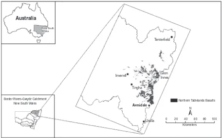
The study area was on the Northern Tablelands of NSW on an area of Tertiary Basalt geology around the township of Guyra (Fig. 1). The soils of the area are Red and Black Ferrosols (Isbell 2002) and have been grouped to form the Northern Tablelands Basalt Soil Monitoring Unit, within the BRG catchment, for the purposes of state-wide soil condition monitoring (Chapmanet al.2009). The altitude across the study area is ~1000 m and the region has a temperate climate with a mean annual rainfall of 880 mm, which is summer-dominant (i.e. total rainfall 108.3 mm in January and 56.1 mm in July). Maximum mean monthly temperatures in January are <308C for all of the selected locations. Mean monthly minimum temperature from April to September is <08C across the sample area and frosts are common (Lodge and Whalley1989).
Site selection
Five‘site clusters’were established on privately owned farms across the study area. On the Northern Tablelands, mixed farming enterprises are typical, and the dominant land-uses are (i) cultivation (for forage, oats, potatoes, and lucerne), (ii) improved pasture (with introduced grass species, legumes, and super-phosphate amendment), (iii) grazing of unimproved native pasture, and (iv) remnant woodland in isolated fragments, roadside reserves, and Travelling Stock Routes. To represent this mix of land uses, each site cluster consisted of 4
Soil sampling
Land-use differences
To measure differences in the selected soil properties between land-use types, 10 soil cores were collected from each treatment at each site cluster. These 10 soil cores were spatially arranged within each 25 by 25 m sample plot (after McKenzieet al.2002), using a random,‘latin square’sampling design. A grid of 100 cells was formed by dividing the 25 by 25 m area into 10 rows by 10 columns. In each column, a cell number from 1 to 10 was selected randomly. This was done for each column in turn but without repeating a cell number in any subsequent column. This ensured complete coverage of the whole area while retaining a random element to the sampling. The nature of each site was also considered (as per McKenzie et al.2002) and stratified on the basis of canopy cover and other distinct vegetation patterns to ensure that the sample cells selected were located in proportion to the site characteristics (e.g. if 20% of the site was under tree canopy cover, then at least 2 of the 10 sample cells were in under-canopy locations). This required occasional modification of the cell selection but in practice this was limited.
Soils were sampled at a random location within the 10 selected 2.5 by 2.5 m cells using a manual coring device of 50 mm diameter, driven into the soil using a wooden mallet to a depth of 300 mm. Previous work in the region (e.g. Wilsonet al. 2002,2008) has illustrated that land-use induced change in soil properties is most strongly expressed in the near surface layers and so, the soil core was subdivided into discrete depth increments (0–50, 50–100, 100–200, and 200–300 mm
depths) in order to elucidate patterns with increasing soil depth. This sampling approach provided samples of known volume which allowed for the subsequent determination of bulk density for each individual sample. At a limited number of sample points, rock was encountered and the 200–300 mm
depth increment could not be sampled.
Optimum sampling intensity
We also wished to determine optimum sampling intensities that would be required to estimate the selected soil parameters using the 25 by 25 m sample plot design, to a given level of precision and confidence. Following McKenzieet al. (2002), the sample sizenwas estimated by:
n¼ t 2 as2
ðxdÞ2
wheretais Student’st-statistic at the level of probabilitya,s2is
the sample variance,xis the sample mean, anddis the desired degree of precision (d%) to estimate the mean. By varying the inputs to this formula (aandd), we can determine the optimum number of samples for each treatment and soil depth. Using this calculation for data generated in this study, estimates were made of the appropriate number of samples required in a 25 by 25 m area on these soils and land uses to a given degree of precision and desired‘half interval’(e.g. (d%).
Nested sampling–sample plot dimensions
We also wished to evaluate the appropriateness of the selected 25 by 25 m plot as recommended in McKenzieet al.
0 20 40 60 80 100 N
Northern Tablelands Basalts
New South Wales
Border Rivers-Gwydir Catchment New South Wales
Australia
Tenterfield
Glen Innes Inverell
Tingha
Armidale
Uralla
Kilometers
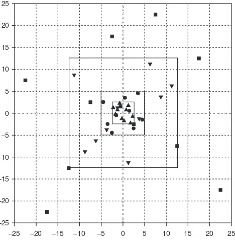
(2000,2002) and Chapmanet al. (2009). For this reason, we selected 2 treatments (woodland and cultivation) at one of our sample locations for intensive spatial sampling with the aim of determining optimum sample plot size. These treatments were selected because it was determined empirically that they provided the two extremes of spatial heterogeneity across the land uses we sampled (woodland highest, cultivation lowest). Other sample area sizes have also been recommended in Australia (e.g. 0.1 ha; McKenzie and Dixon 2006). To accommodate and test the suitability of a range of sampling plot sizes, soil sampling was therefore undertaken following a nested design using a series of concentrically arranged sample
squares of 5 by 5 m (0.0025 ha), 10 by 10 m (0.01 ha), 25 by 25 m (0.0625 ha), and 50 by 50 m (0.25 ha) plots (Fig.2). Each sample plot was divided into 100 cells and sampled using the random,‘latin square’sampling design described above. This sampling allowed for an analysis to determine the statistical efficiency of sampling at each spatial scale and therefore the most appropriate sample plot dimensions across the land uses sampled.
Soil analysis
Soil samples were stored in cool (<58C) dark conditions until they could be processed. Samples were dried at 408C for 48 h Table 1. Site characteristics and management history of sample sites across the Basalt landscape of north-west New South Wales
Site Land use Soil type Time under regime Management
Guyra 1 365203E
6662233N
Cultivation Black Ferrosol >30 years Cropped, now sown to triticale for grazing lambs. History of crop/pasture
rotation. N fertiliser 365123E
6662347N
Improved Pasture Black Ferrosol >5 years Sown to pasture>5 years ago. Grazed since then. Light superphosphate
application at sowing. No subsequent fertiliser application 365538E
6662284N
Unimproved Pasture Black Ferrosol >20 years Roadside reserve. Native grass. Lightly and periodically grazed. Never
cultivated. No fertiliser 365315E
6662290N
Woodland Black Ferrosol >100 years Roadside reserve. Grassy eucalypt woodland, native grass cover, lightly and
periodically grazed. Never cleared. No fertiliser
Guyra 2 366801E
6659753N
Cultivation Black Ferrosol >15 years Cultivated at 3-yearly intervals (most recently 2008). Oats. N, P, K
application at sowing with follow upNapplication 367169E
6659969N
Improved Pasture Black Ferrosol >10 years Sown fescue, ryegrass, clover pasture. Lightly grazed. Regular
superphosphate at sowing and subsequently every 2 years 366796E
6659580N
Unimproved Pasture Black Ferrosol >30 years Native grass. Lightly and periodically grazed. Never cultivated. Light
superphosphate application 367699E
6659717N
Woodland Black Ferrosol >100 years Roadside reserve. Grassy eucalypt woodland, native grass cover, lightly and
periodically grazed. Never cleared. No fertiliser
Black mountain 1 369222E
6647986N
Cultivation Red Ferrosol >15 years Cultivated for potatoes and forage. Minimal fertiliser application
369240E 6647810N
Unimproved Pasture Red Ferrosol >50 years Native grass. Lightly and periodically grazed. Never cultivated. No fertiliser
396308E 6647881N
Woodland Red Ferrosol >100 years Remnant woodland. Grassy eucalypt woodland, native grass cover, lightly
and periodically grazed. Never cleared. No fertiliser
Black mountain 2 371664E
6645933N
Cultivation Black Ferrosol >20 years Cropped with millet. History of crop/pasture rotation. Had 0.5 t/ha lime
applied ~5 years before sampling 371391E
6645969N
Improved Pasture Black Ferrosol <20 years Sown with mixed improved pasture (red clover–rye grass–phalaris). 0.5 t/ha
lime applied ~5 years before sampling 371498E
6646093N
Unimproved Pasture Black Ferrosol >100 years Native grass. Lightly and periodically grazed. Never cultivated. No fertiliser
371400E 6646091N
Woodland Black Ferrosol >100 years Roadside reserve. Grassy eucalypt woodland, native grass cover, lightly and
periodically grazed. Never cleared. No fertiliser
Black mountain 3 371664E
6645933N
Cultivation Black Ferrosol >20 years Cropped with millet. 0.5 t/ha lime applied ~5 years before sampling
371391E 6645969N
Improved Pasture Black Ferrosol >20 years Sown with improved pasture species ~10 years before sampling. Beginning
to revert to native perennial pasture. Gypsum topdressed ~5 years before sampling
371498E 6646093N
Unimproved Pasture Black Ferrosol >100 years Native grass. Lightly and periodically grazed. Never cultivated. No fertiliser
371400E 6646091N
Woodland Black Ferrosol >100 years Roadside reserve. Grassy eucalypt woodland, native grass cover, lightly and
(after Wilsonet al.2009), then crushed to pass a<2-mm sieve. Bulk density was determined on each individual sample. Each sample was then analysed for pH(1 : 5 CaCl2) and total carbon
and nitrogen using LECO dry combustion (ASPAC Method Code CA-37) at the Environmental Analysis Laboratory, Southern Cross University, Lismore. Soil carbon densities (to 300 mm soil depth) were calculated as a product of the measured carbon (%), bulk density, and soil depth for each individual sample from the various land uses. In order to compare carbon densities between land uses, it is now generally considered appropriate to calculate carbon densities between different land uses. This was done for the soils sampled and results expressed as an equivalent soil mass to 300 mm depth (see Ellertet al.2001).
Statistical analysis Land-use effects
Data collected from each treatment at each site (25 by 25 m sample plot) were analysed using a repeated-measures analysis of variance (GENSTAT 2008). Since depth observations were
taken at non-equally spaced intervals (0–50, 50–100,
100–200, 200–300 mm), a power model was used to investigate the correlation of the residuals as being dependent upon the distance between depths calculated from their midpoints (25, 75, 150, 250 mm). Heterogeneity of variances was also catered for in the analysis, based on residual plots indicating variance increasing over depth. To satisfy requirements for normality, a rescaling transformation (100 * log e{x+ 1}) was necessary for carbon and nitrogen. Significance of the fixed effects of land use, depth, and their interaction was examined using approximateFstatistics. Since this interaction was always significant, depth profiles were graphed for each land use, and means compared using l.s.d.
(P<0.05). Differences between total carbon density (T/ha) were determined using one-way ANOVA andpost-hocl.s.d. analysis (P<0.05).
Optimum sample numbers
From the data generated across the 5 site clusters, sample numbers were calculated that would be required to achieve given levels of precision (i.e. d%) at a set level of confidence (a= 0.1). These data were calculated based upon the measured variance of the property measured across the 25 by 25 m plot.
Nested sampling
The statistical efficiency of sampling at each spatial scale was compared by summarising the 10 data values from each of 4 plot sizes, and repeated using 4 depths from the 2 selected land uses. Efficiency was judged by comparing the standard error of the observed mean, expressed as a percentage of the mean in order to standardise across potentially changing scales.
Data were merged across the 4 nested plots to form an XYZ dataset of 40 values identified by unique 2-dimensional spatial coordinates (distance in meters from the south-west corner of the largest plot to the soil core site). Spatial variation was characterised by forming the variogram (Webster and Oliver 2001) for each variate from separate depths and management units. A variogram attempts to quantify the expectation that values of a soil variable at 2 locations close together will generally be similar (i.e. low variance, high correlation), whereas the values at more widely separated locations will be less similar (higher variance, lower correlation). In order to construct the variogram, the variance between all pairs of spatially located points was determined. The physical distance between each pair of points (the ‘lag’ distance) was also calculated and grouped into suitable classes and the set of variances of those pairs of points that comprise each distance group were averaged. Each variogram was then constructed to provide a graphical representation of the trend in average variance of pairs of soil sampling points, the points having been grouped into sets, with increasing lag distances apart.
The shape of the variogram helps interpret how the variance of the property of interest changes over spatial distance. It might be expected that the variogram curve will pass through the origin of the graph since soil samples from sites infinitely close together (lag distance = 0) would be expected to have zero variance. Variograms constructed from sample data, however, showed a positive non-zero variance as the lag distance approached zero. The size of this non-zero variance is known as the nugget variance and represents the inherent variation at distances smaller than the sample spacing including measurement error.
Results
Land-use effects on soil properties
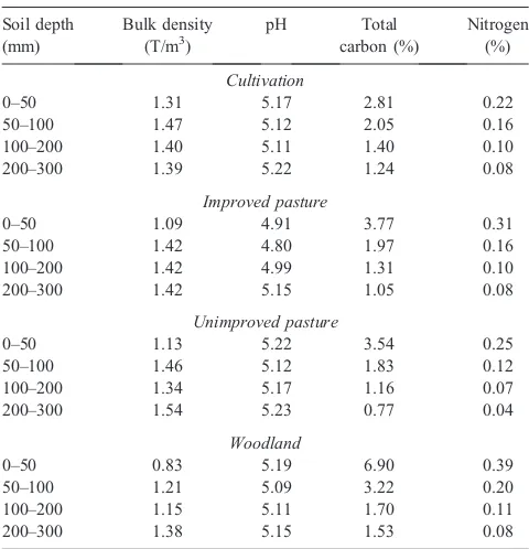
Soil properties differed between the 4 land-use types examined (Table 2). When all the data for all sites, land uses, and soil depths were considered in an ANOVA, a significant (P<0.05) land-use effect was found only for soil bulk density (Table 3), with woodland bulk densities being significantly
–25 –20 –15 –10 –5 0 5 10 15 20 25 –25
–20 –15 –10 –5 0 5 10 15 20 25
lower at all soil depths compared with the other land-use types. No significant main-order land-use effect was observed for soil pH, carbon, and nitrogen.
All soil properties determined showed a significant (P<0.001) depth effect (Table 3), indicating that soil properties differed significantly between the soil depths sampled. Bulk density was typically lower in the surface soil layers compared with deeper soils (Table 2). Soil pH was significantly (P<0.05) lower in the 50–100 and 100–200 mm layers than other soil layers, across all land uses sampled, while carbon and nitrogen both declined with increasing soil depth.
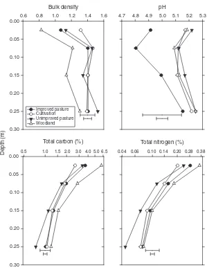
A strongly significant (P<0.001) land usedepth interaction was also found for all soil properties determined, indicating different depth profile characteristics between land uses (Table3). Examination of the plots of soil properties with depth (Fig.3) indicates that soil pH was significantly lower at all soil depths under improved pasture compared with all other land uses. For carbon, however, woodland had significantly higher values in the surface layers (0–50 and 50–100 mm) compared
with all other land uses (P<0.05 using l.s.d.post-hoc). In the 0–50 mm layer, the improved and unimproved pasture sites had
similar carbon levels but both were larger than the cultivation land use. Woodland soils also had significantly higher nitrogen content than all other land uses at 0–50 mm. Below these depths,
however, no significant difference existed between the land uses except for slightly but significantly (P<0.05) lower
carbon and nitrogen concentration under unimproved pasture at 200–300 mm.
Soil carbon densities (to 300 mm soil depth) were also calculated for each land use across the study area (Table 4); woodland had a larger quantity of soil carbon to 300 mm depth than unimproved pasture only (Table4). However, when carbon density was expressed on an equivalent mass basis, woodland carbon density was significantly higher than all other land uses but there remained no significant difference in carbon density between the other land uses.
Determination of optimum sample numbers
We also wished to determine optimum sampling intensities that would be required to estimate the selected soil parameters using the 25 by 25 m sample plot design, to a given level of precision and confidence. The suggested half interval values (i.e. 5, 10, 15, and 20%) in Table5have been drawn from the literature and the likely magnitude of‘important’changes in soil properties (i.e. between land uses, what level of difference we might expect in soil properties). For example, Schipper and Sparling (2000) suggested that for soil condition monitoring, an appropriate level of precision might be10% of the mean at a confidence level of 90%. For this reason, level of confidence in Table5has been held constant at 90% throughout while the level of precision has been manipulated to provide indicative sample numbers.
The various soil properties had very different variances associated with the data generated and therefore had different sample numbers required to achieve the defined levels of precision and confidence (i.e. d%, 90% of the time). Soil pH measurement for example, required relatively few samples across the site to achieve relatively high levels of precision and confidence (Table 5). These sampling requirements differed little between the land uses, rising to a maximum of 6 samples for woodland at the highest level of precision (5%). For the other properties measured, however, the sampling intensity required to achieve desired levels of confidence were considerably higher and varied a great deal with land use and sampling depth. For soil bulk density, large numbers of samples would be required to achieve a precision of 5%; however, these sampling numbers declined to reasonable sample numbers at the 15% level. For carbon and nitrogen, similar patterns were found. Sample numbers required to achieve5% precision were generally very large and were typically lowest for cultivation sites and largest for woodland sites, with pasture sites being intermediate. As with bulk density, however, reasonable sample numbers were determined if the 15% precision level was met.
In most cases, larger sample numbers were required to estimate soil properties in the 200–300 mm soil layer
compared with shallower soil layers, with the exception of Table 2. Mean values for each land-use type
Soil depth Bulk density pH Total Nitrogen
(mm) (T/m3) carbon (%) (%)
Cultivation
0–50 1.31 5.17 2.81 0.22
50–100 1.47 5.12 2.05 0.16
100–200 1.40 5.11 1.40 0.10
200–300 1.39 5.22 1.24 0.08
Improved pasture
0–50 1.09 4.91 3.77 0.31
50–100 1.42 4.80 1.97 0.16
100–200 1.42 4.99 1.31 0.10
200–300 1.42 5.15 1.05 0.08
Unimproved pasture
0–50 1.13 5.22 3.54 0.25
50–100 1.46 5.12 1.83 0.12
100–200 1.34 5.17 1.16 0.07
200–300 1.54 5.23 0.77 0.04
Woodland
0–50 0.83 5.19 6.90 0.39
50–100 1.21 5.09 3.22 0.20
100–200 1.15 5.11 1.70 0.11
200–300 1.38 5.15 1.53 0.08
Table 3. Fstatistics andPvalues from the analysis of variance of soils from the Northern Tablelands Basalts
Bulk density pH Total carbon Total nitrogen
F P F P F P F P
Land-use 13.05 0.005 0.66 0.592 3.05 0.074 1.64 0.222
Depth 262.03 <0.001 23.64 <0.001 609.38 <0.001 709.73 <0.001
improved pastures. These numbers reflect a larger variance at these depths. However, although the variance as a proportion of the mean was larger, this must be placed in the context of the relatively small values for soil carbon and nitrogen that were found at these depths. That is, a large variance in carbon and nitrogen value at these depths actually reflects relatively small absolute values.
Nested sampling
Variance of the datasets for each plot size under each land use was expressed as a standard error of the mean (s.e.m.) and is presented as a percentage of the mean (Table 6). Analysis of these data indicate that the s.e.m. for all properties examined was considerably and consistently larger for all plot sizes and soil depths under woodland compared with cultivation (with only 1 exception: nitrogen, 5 by 5 m, 0–50 mm).
There were considerable differences in the level of variability among the soil properties examined. For example, soil pH consistently had lower levels of variability than the other soil properties (Table6). Soil carbon and nitrogen typically had the highest levels of variability and again this was especially so in the deeper soil layers.
Within the cultivation and the woodland datasets, there were no clear or consistent patterns in the variability between plot sizes and no specific plot size appeared to contain more variability than the others.
pH
4.7 4.8 4.9 5.0 5.1 5.2 5.3 Bulk density
0.6 0.8 1.0 1.2 1.4 1.6
Depth (m)
0.00
0.05
0.10
0.15
0.20
0.25
0.30
Improved pasture Cultivation Unimproved pasture Woodland
Total carbon (%)
0.5 1.0 1.5 2.0 3.0 4.0 5.0 6.5
Total nitrogen (%)
0.04 0.06 0.10 0.14 0.20 0.28 0.38 0.00
0.05
0.10
0.15
0.20
0.25
0.30
Fig. 3. Plots of soil parameters by depth across land uses.*Improved pasture,*cultivation, !unimproved pasture,~woodland. The larger l.s.d. bar compares means across land use and depth, the smaller compares depths for a specific land use. Note the nonlinear scale for carbon and nitrogen due to their need for transformation.
Table 4. Total carbon density to 300 mm (T/ha, calculated and expressed as equivalent mass) for all land-uses
Within columns means followed by the same letter are not significantly different atP= 0.05
Calculated Corrected for equiv. mass
Cultivation 70.3ab 70.3a
Improved pasture 68.1ab 68.9a
Unimproved pasture 60.8b 60.8a
Modelling the variograms formed by the aggregation of data from the 4 levels of nested sampling generally proved to be unsuccessful (Fig.4). The exponential modelfitted carbon in the 0–50 mm layer of woodland (R2= 0.69), and weakly so for
cultivation land use (R2= 0.27). The reasonably large nugget variance shown for carbon suggests that for this soil property, relatively high variances exist at spatial scales 5 m. With limited confidence, the interpretation of the rising curve for soil carbon in woodland implies that dependence between samples continues over a larger spatial scale when compared to the more asymptotic cultivation curve over the same distances. For all other variables from sampled depths and land uses, the exponential model, and all other models attempted, failed to fit any of the remaining datasets (Fig.4). While invaluable for comparing sampling configuration, the nested arrangement of sampling points (Fig. 2) may have hindered the ability to confidently estimate these variograms. As noted by Webster and Oliver (2001), a regular sampling grid is most desired for variogram estimation and mapping.
Discussion Land-use effects
Several significant patterns and trends were found in the data from the various land-use types and sites across the Northern Tablelands Basalts. Soil bulk density had a significant land-use effect and was significantly lower under woodland compared with all other land-use types. This is a commonfinding in this region and is indicative of generally higher organic matter contents and soil porosity under trees compared with other land-uses (Graham et al. 2004; Young et al. 2005; Wilson et al. 2008). For all soil properties, however, a strong, significant depth effect and land usedepth interaction was found, which we interpret to indicate that differences in the various soil properties between land uses were restricted to the
surface soil layers (Fig.3). Differences between land uses for the various soil properties diminished with soil depth and by 200–300 mm depth, differences between land uses were
undetectable. This result confirms the findings of other work from this region (Younget al.2005; Wilsonet al.2008) and elsewhere (Dalal and Chan2001).
Where these differences between land uses were found, woodland had higher pH, carbon, and nitrogen contents and lower bulk density compared with all other land-use types, a result which again conforms with other work in this region (e.g. Wilsonet al.2008). Much of the woodland within the study area was cleared during the late 18th and early 19th Centuries in order to develop land for agriculture (Reid et al. 1997). Surviving woodland in the region therefore tends to represent little modified and minimally managed sites by comparison with the remainder of the cleared landscape. The consistently higher concentration of carbon and nitrogen and higher pH of these sites might therefore provide an insight into the potential pre-clearing soil condition in the region and indicate the value of this land use as a‘reference’against which other soils and land uses might be compared.
Soil properties between the other, non-woodland land-use types were largely similar apart from the very strong acidity under improved pasture. This was particularly so in the 50–100 mm layer of these pasture soils, which is the zone of
legume root activity and therefore potential nitrogen leaching. This process has been well documented in its association with soil acidification (e.g. Helyar and Porter 1989; Lockwood et al. 2003; Rengel 2003). Soil pH in the 50–100 mm layer of these improved pasture soils was found to be as low as 4.8, a significant threshold below which plant growth and potentially pasture productivity can be impaired (Lockwoodet al.2003). This result is all the more surprising given the clay-rich, basalt soils that are commonly believed to Table 5. Number of samples required per 25 by 25 m plot to estimate mean within half intervalsþd% at 90% confidence (P= 0.1)
Depth pH (mean ±d%) Bulk density (mean ±d%) Nitrogen (mean ±d%) Carbon (mean ±d%)
(mm) 5% 10% 15% 20% 5% 10% 15% 20% 5% 10% 15% 20% 5% 10% 15% 20%
Cultivation
0–50 3 1 1 1 52 13 6 3 41 10 5 3 34 8 4 2
50–100 4 1 1 1 38 9 4 2 66 16 7 4 49 12 5 3
100–200 1 1 1 1 20 5 2 1 65 16 7 4 62 16 7 4
200–300 1 1 1 1 43 11 5 3 134 33 15 8 154 39 17 10
Improved pasture
0–50 2 1 1 1 54 13 6 3 90 22 10 6 88 22 10 6
50–100 1 1 1 1 12 3 1 1 95 24 11 6 66 17 7 4
100–200 1 1 1 1 14 3 2 1 45 11 5 3 36 9 4 2
200–300 1 1 1 1 19 5 2 1 73 18 8 5 80 20 9 5
Unimproved pasture
0–50 2 1 1 1 41 10 5 3 68 17 8 4 89 22 10 6
50–100 1 1 1 1 22 5 2 1 67 17 7 4 178 44 20 11
100–200 2 1 1 1 57 14 6 4 59 15 7 4 54 13 6 3
200–300 1 1 1 1 32 8 4 2 98 24 11 6 93 23 10 6
Woodland
0–50 6 2 1 1 55 14 6 3 126 32 14 8 191 48 21 12
50–100 3 1 1 1 30 8 3 2 157 39 17 10 316 79 35 20
100–200 2 1 1 1 91 23 10 6 125 31 14 8 178 45 20 11
be well buffered against acidification (Lockwoodet al.2003). Our results therefore suggest that soil carbon and nitrogen increased modestly under improved pasture in this region compared with other non-wooded land uses but that this soil change was associated with a significant and potentially damaging reduction in soil pH.
The low levels of carbon and nitrogen in cultivated soils compared with woodland is to be expected and is widely reported (e.g. Murphy et al. 2002), resulting from soil disturbance and mineralisation of organic matter in the surface soil. However, in our study, the soils of all non-wooded land uses were statistically similar. There was no evidence that any of the native pasture sites that we studied had a history of cultivation or similar soil disturbance, so this result suggests that management, whether it be cultivation, pasture improvement, or prolonged grazing, will result in organic matter depletion in these environments relative to woodland systems.
Given the recent interest in land-use types and potential carbon storage, we also calculated the carbon density (to
300 mm) across the various land uses examined. When the carbon density was corrected for equivalent mass (after Ellert et al. 2001), using cultivated soils as the standard mass, the woodland sites had a significantly (P<0.05) larger quantity of carbon than any other land use, while the other land uses remained statistically similar. On an equivalent mass basis, the woodland soils contained, on average, 28 T/ha more carbon than any other land-use sampled. Comparing the various land use systems sampled, it is therefore clear that in order to maintain the largest quantity of carbon in the landscape of the study area, retaining trees and woodland is the most effective option.
Optimum sample numbers
The data collected also provided a useful insight into sampling efficiency and the estimation of optimum sampling numbers to guide future sampling strategies. The data for optimum sample numbers suggest that, overall, the variability of soil pH was considerably lower than that of the other soil properties. Therefore, if the intention of monitoring was to estimate soil pH alone, this would require relatively few samples to estimate pH to a high level of precision. Schipper and Sparling (2000) suggested that for soil condition monitoring, an appropriate level of precision might be10% of the mean at a confidence level of 90%. For all land uses and all soil depths, this level of precision and confidence could be met for pH by collecting no more than 2 samples per 25 by 25 m sample plot (Table5). However, in practice, the number of samples required will be limited by the most variable soil property that is to be estimated, and in our study, bulk density, carbon, and nitrogen were all considerably more variable. The greater degree of variability in bulk density and carbon compared with pH conforms to results generated at a quite different range of sites and soil types in NSW by Wilson et al. (2007) and Chapmanet al. (2007).
In addition, different land uses and soil depths showed a different level of variability. For example, in all cases, the variability of soil carbon was considerably higher under woodland than other land uses and also generally at depth than in the near-surface layers. This result conforms to those of other studies in the region (Younget al.2005; Wilsonet al. 2008). For soil bulk density, carbon, and nitrogen, optimum sample numbers were therefore rather large (if not prohibitive at higher levels of precision) for several land-use/depth combinations. Our results, however, indicate that the required sample numbers became achievable for these soil properties at a precision level of15% for virtually all land uses near to the soil surface, with the exception of woodland soils, which were considerably more variable. In the deeper soil layers, the large variance that was found for some soil properties can be attributed to variation in what are actually very small values, and we believe that the large sample numbers suggested in Table5would, in practice, be unnecessary.
McKenzie et al. (2000, 2002) suggested that 25 samples should be collected across a 25 by 25 m square, bulked to 5 samples for analysis. This approach, they propose, would allow us to account for variability across a site while reducing sample numbers for analysis. However, our results suggest that using 25 samples would only marginally improve the level of precision Table 6. Standard error of the mean (expressed as a percentage of the
mean) across all 10 samples for each sample plot size
Plot size Depth
100–200 2.0 9.7 10.6 4.6
200–300 1.2 7.1 9.5 6.5
25 by 25 m 0–50 2.5 11.4 6.3 3.5
50–100 2.0 18.9 9.6 5.4
100–200 2.0 28.1 15.9 5.3 200–300 1.6 15.0 15.8 4.9
50 by 50 m 0–50 1.4 7.3 5.8 4.6
50–100 2.3 7.1 6.4 6.3
100–200 1.6 10.4 9.3 6.1
and only for some land uses and soil depths. Overall, we believe that the increased logistical input required, over large numbers of sites in a monitoring program, would not justify this modest improvement in precision. Problems also exist with respect to bulking, in that it limits our ability to compute the level of variability across the site to inform subsequent sampling campaigns. We therefore suggest that 10 samples across a site 25 by 25 m generates an adequate level of precision with a reasonable sampling effort and that each sample should be analysed separately, at least in thefirst stages of a monitoring program, in order to clearly define the level of precision and confidence for the purposes of reporting.
Given this information, what might be the implications for future sampling design? We propose that if we aim to use these data to inform the future sampling protocol, and to minimise unnecessary sampling effort (i.e. bulk samples on site), we are faced with 3 alternative responses:
(i) We might set a standard number of samples and be aware that the degree of precision will vary between land uses and depths. For example, mean values generated in cultivation might have a level of precision that is considerably higher than for woodland sites. This need not be a significant problem if the intent is simply to track broad trend across the landscape. However, if we wish to generate a statistically robust dataset, this might undermine our confidence in the data to a significant degree. (ii) Alternatively, we could relax our desired level of precision and confidence (i.e.15% of the mean, 90% of the time) and modify the sample number appropriately. This would provide a robust dataset but would require considerable logistical input since sample numbers would need to be adjusted by land use, soil depth, etc. Sampling a large number of soils across a 25 by 25 m plot is demanding
in time. Extrapolated across a landscape or monitoring region, the cost could be significant.
(iii) As a third option we might consider the‘real’values that are represented by the calculated percentage half intervals. For example, 10% of a mean soil carbon value of 4.35% is 0.44%. This is not a large number and might be considered sufficient to satisfy our reporting needs. This judgement depends upon the required level of precision, i.e. what difference do we hope to detect? This issue is especially pertinent to deeper samples. Soil carbon diminished significantly with depth and percentage half intervals therefore become progressively smaller in ‘real’
magnitude. It is also less likely that we will detect significant change in soil carbon at these depths resulting from management treatment. At these depths, a larger half interval might therefore be acceptable for our needs.
Despite the varying requirements for optimum sampling numbers across the sample sites, we were able to detect strong and significant land-use effects on the soil properties determined. There was, however, a limited statistical difference between the non-wooded land uses in some properties, especially total carbon. This result might suggest that no difference existed between these land uses (although significant differences have been reported elsewhere, e.g. Wilsonet al.2008). However, it might also be that more intense sampling might have detected such differences. The decision as to sampling intensity is therefore one of a compromise between efficiency and purpose of the data generated.
Nested sampling
Several sampling approaches have been recommended in the published literature recently (e.g. McKenzieet al.2000,2002,
0 5 10 15 20 25 0 5 10 15 20 25
0 5 10 15 20 25 pH
pH
Carbon %
Carbon %
Nitrogen %
Nitrogen % Cultivation
Woodland
Lag distance (m)
V
ar
iance
2008; McKenzie and Dixon2006; Chapmanet al.2007; Wilson et al.2007) and each suggests specific sample area and design for a range of (often arbitrary) reasons. For example, McKenzie et al. (2000) recommended a minimum 400 m2 area for soil sampling in order to accommodate a range of soil variability, including that imposed by mature trees. McKenzieet al. (2000, 2002,2008) went on to suggest the use of a 25 by 25 m sampling area (625 m2) to conform to the then pixel size of remote imaging technologies. In contrast, McKenzie and Dixon (2006) and Skjemstadet al. (2006) considered that a minimum of 0.1 ha sample area would be required to adequately account for soil variability and provide sufficient confidence for soil monitoring across Australia.
Our nested sampling indicated that the variance (as a percentage of mean) differed little between sample plot sizes for the woodland and cultivation sites studied. These two land uses were selected, from our larger dataset and pre-existing data (Wilsonet al.2007), to represent the most and least variable land-use types. Although woodland soils were consistently more variable, the pattern of variance between the sample plot sizes persisted across both land uses. This result suggests that the size of sample plot had little effect on the variability of the result generated in either land-use.
Similar studies have been conducted elsewhere with different results. For example, Lark (2005) measured a range of soil properties across nested spatial scales and found scale dependence for some soil properties, notably bulk density, pH, and extractable phosphorus at spatial distances up to 50 m. However, von Steiger et al. (1996) found such spatial dependence for soil carbon only up to 15 m. There is a common belief that increasing spatial scale of sampling will inevitably result in an increasing degree of variability, and previous studies have suggested that this will result over finite distances. However, our results appear to indicate that no such spatial dependence existed at the sites and soils we studied. Prior sampling and knowledge of spatial variability therefore allows for the assessment of the suitability of the sampling approach and for account to be made of any spatial dependence in the data generated. In our study, the indication is that, within the spatial range we tested, the sample area size selected for soil measurement is largely arbitrary. Nevertheless, for repeat sampling and regional and national consistency, selection and standardisation on one such area would be preferred. Since much work in Australia has already been conducted using the 25 by 25 m sampling area approach (McKenzieet al.2000, 2002; Murphy et al.2002; Chapman et al. 2009), we recommend that this area be continued as a standard approach for soil monitoring in Australia.
It is acknowledged that this study was undertaken at only 5 properties and one soil monitoring unit across a relatively large region. However, the properties and sample sites selected were believed to be representative of the region. For the purposes of broad-scale monitoring, preliminary examination of a wider range of sites, soil types, and land uses would be necessary to definitively determine appropriate sampling strategies. This process has begun under the NSW Land and Soil Condition Monitoring Program, coordinated by the NSW Department of Environment, Climate Change and Water.
Conclusions
Land-uses had a profound impact on soil properties near to the soil surface. Even with the large within-site variability at the sites studied, significant land-use effects were found for the range of soil properties examined. This was particularly true of the near-surface soil layers. Woodland soils in this environment had consistently higher values for carbon and nitrogen and lower bulk density in the surface soil layers.
Data for soil carbon assessment should account for equivalent mass since this significantly modifies carbon densities, particularly for the lighter, woodland soils. Soil carbon density (corrected for equivalent soil mass) was consistently and significantly higher under woodland compared to all other land-use types, and in order to maintain the largest quantity of carbon in this landscape, retaining trees and woodland is the most effective option.
Analysis of spatial variability of sampling sites for monitoring allows us to make informed decisions regarding sampling intensity and the precision and confidence of soil property estimation. The required soil sampling intensity to achieve defined outcomes of precision and confidence differed between the land uses and soil properties examined. Broadly, 10 samples across a sample area 25 by 25 m were sufficient to estimate most soil properties to within 15% at 90% confidence at the sites and soil types we studied. We believe that, on the basis of our results, similar sampling principles can be applied more broadly across the landscapes of NSW.
Selection of a sampling area size across a range of recommended dimensions suggests that sampling size is largely arbitrary. The most significant recommendation with respect to sample area size is that it should be consistent to promote comparability of existing and future datasets.
Acknowledgments
The authors gratefully acknowledge the assistance of the various landholders across the Northern Tablelands for their assistance in accessing and establishing soil monitoring and research sites. We also acknowledge the funding support of the NSW Department of Environment, Climate Change and Water through the Statewide Land and Soil Condition Monitoring Program. Special thanks are extended to Greg Chapman, Peter Barker, and Brian Murphy for constructive comments on the work reported. Thanks also to ananymous referees for constructive comments on our original manuscript.
References
Chan KY (2001) Soil particulate organic carbon under different land use management.Soil Use and Management14(4), 217–221. doi:10.1079/ SUM200180
Chan KY, Heenan DP, Oates A (2002) Soil carbon fractions and relationship to soil quality under different tillage and stubble management.Soil & Tillage Research 63(3–4), 133–139. doi:10.1016/S0167-1987(01) 00239-2
Chapman G, Murphy B, Bowman G, Wilson B, Jenkins B, Koen T, Gray J, Morand D, Atkinson G, Murphy C, Murrell A, Milford H (2009)‘NSW soil condition monitoring: soil carbon, soil pH, soil structure, ground cover & land management–Protocols for initial MER soil sampling.’ (Ed. G Bowman) (Scientific Services Division, NSW Department of Environment and Climate Change: Sydney)
Chapman GA, Davy M, Symes L, Yang X, Wilson BR (2007) Report on Indicator Protocol Trial for Soil Acidity Monitoring, NSW. Report to the National Land and Water Resources Audit, National Monitoring and Evaluation Framework, Canberra, July 2007.
Chilcott C, Reid N, King K (1997) Impact of trees on the diversity of pasture species and soil biota in grazed landscapes on the northern Tablelands, NSW. In‘Conservation outside nature reserves’. (Eds P Hale, D Lamb) (Centre for Conservation Biology, University of Queensland: Brisbane) Collard SJ, Zammit C (2006) Effects of land-use intensification on soil carbon and ecosystem services in Brigalow (Acacia harpophylla) landscapes of southeast Queensland, Australia.Agriculture, Ecosystems & Environment
117(2–3), 185–194. doi:10.1016/j.agee.2006.04.004
Dalal RC (1989) Long-term effects of no-tillage, crop residue, and nitrogen application on properties of a Vertisol.Soil Science Society of America Journal53, 1511–1515.
Dalal RC, Chan KY (2001) Soil organic matter in rainfed cropping systems of the Australian cereal belt.Australian Journal of Soil Research39, 435–464. doi:10.1071/SR99042
de Gruijter JJ, Brus D, Bierkens M, Knotters M (2006)‘Sampling for natural resource monitoring.’(Springer: Berlin)
Doran JW (1996) Soil quality and health: the international situation and criteria for indicators. In ‘Proceedings, Workshop on Soil Quality Indicators for New Zealand Agriculture’. 8–9 February 1996. (Lincoln University: Christchurch, New Zealand)
Ellert BH, Janzen HH, Entz T (2002) Assessment of a method to measure temporal change in soil carbon storage.Soil Science Society of America Journal66, 1687–1695.
Ellert BH, Janzen HH, McConkey B (2001) Measuring and comparing soil carbon storage. In‘Assessment Methods for Soil Carbon’. Advances in Soil Science. (Eds R Lal, JM Kimble, RF Follet, BA Stewart) (Lewis Publishers: Boca Raton, FL)
Farquharson RJ, Schwenke GD, Mullen JD (2003) Should we manage soil organic carbon in Vertosols in the northern grains region of Australia? Australian Journal of Experimental Agriculture 43(3), 261–270. doi:10.1071/EA00163
GENSTAT(2008)‘The guide to GENSTATRelease 11. Part 2: Statistics.’(VSN International: Hemel Hempstead, UK)
Graham S, Wilson BR, Reid N (2004) Scattered paddock trees, litter chemistry and surface soil properties in pastures of the New England Tablelands, NSW.Australian Journal of Soil Research42, 905–912. doi:10.1071/SR03065
Greenwood KL, McKenzie BM (2001) Grazing effects on soil physical properties and the consequences for pastures: a review. Australian Journal of Experimental Agriculture 41, 1231–1250. doi:10.1071/ EA00102
Harms B, Dalal R, Wang W (2004) Soil carbon and soil nitrogen changes after clearing of mulga vegetation. In ‘Supersoil: Annual Conference of the Australian Soil Science Society and the New Zealand Soil Science Society’. Sydney, 5–9 December 2004. (ASSSI: Sydney)
Harte AJ (1984) Effect of tillage on the stability of three red soils of the northern wheatbelt.Journal of Soil Conservation40, 94–101. Helyar KR, Porter W (1989) Soil acidification, its measurement and the
processes involved. In‘Soil acidity and plant growth’. (Ed. AD Robson) pp. 61–101. (Academic Press: Sydney)
Isbell R (2002)‘The Australian Soil Classification.’(CSIRO Publishing: Melbourne)
Jackson J, Ash AJ (2001) The role of trees in enhancing soil nutrient availability for native perennial grasses in open eucalypt woodlands of north-east Queensland. Australian Journal of Soil Research 52, 377–386.
Jones RJA, Verheijen FGA, Reuter HI, Jones AR (Eds) (2008) ‘Environmental assessment of soil for monitoring. Vol. V: Procedures & Protocols.’EUR 23490 EN/5. (Office for the Official Publications of the European Communities: Luxembourg)
Karlen DL, Mausbach MJ, Doran JW, Cline RG, Harris RF, Schumann GF (1997) Soil quality: a concept, definition and framework for evaluation. Soil Science Society of America Journal61, 4–10.
Lark RM (2005) Exploring scale-dependent correlation of soil properties by nested sampling.European Journal of Soil Science56(3), 307–317. doi:10.1111/j.1365-2389.2004.00672.x
Lockwood PV, Wilson BR, Daniel H, Jones M (2003)‘Soil acidification and natural resource management: directions for the future.’(University of New England: Armidale, NSW)
Lodge GM, Murphy SR, Harden S (2003a) Effects of grazing and management on herbage mass, persistence, animal production and soil water content of native pastures. 1. A redgrass-wallaby grass pasture, Barraba, North West Slopes, New South Wales. Australian Journal of Experimental Agriculture 43, 875–890. doi:10.1071/ EA02188
Lodge GM, Murphy SR, Harden S (2003b) Effects of grazing and management on herbage mass, persistence, animal production and soil water content of native pastures: 1. A mixed native pasture, Manilla, North West Slopes, New South Wales. Australian Journal of Experimental Agriculture 43, 891–905. doi:10.1071/ EA02189
Lodge GM, Whalley RBD (1989) Native and natural pastures on the Northern Slopes and Tablelands of New South Wales. Technical Bulletin 35, NSW Agriculture and Fisheries.
McKenzie NJ, Dixon J (2006) Monitoring soil condition across Australia: recommendations from the expert panel. Prepared on behalf of the National Coordinating Committee on Soil and Terrain, National Land and Water Resources Audit, Canberra.
McKenzie NJ, Grundy MJ, Webster R, Ringrose-Voase AJ (2008) ‘Guidelines for Surveying Soil and Land Resources.’ 2nd edn (CSIRO Publishing: Melbourne)
McKenzie NJ, Henderson B, McDonald W (2002) Monitoring Soil Change: Principles and practices for Australian conditions. CSIRO Land and Water, Technical Report 18/02, CSIRO, Canberra.
McKenzie NJ, Ryan PJ, Fogarty P, Wood J (2000) Sampling, measurement and analytical protocols for carbon estimation in soil, litter and coarse woody debris. National Carbon Accounting System Technical Report No. 14, September 2000, Australian Greenhouse Office, Canberra.
Murphy BW, Rawson A, Ravenscroft L, Rankin M, Millard R (2002) Paired site sampling for soil carbon estimation–NSW. Australian Greenhouse Office Technical Report No. 34, Canberra.
NRC (2005) Standard for Quality Natural Resource Management. New South Wales Natural Resources Commission, Sydney, Australia, September 2005.
Packer I, Medway J, Jones B, Koen T (1998) Are‘conservative’cropping systems improving soil infiltration, organic carbon and bulk density in southern NSW. In ‘Proceedings of the 9th Australian Agronomy Conference’. Charles Sturt University, Wagga Wagga, NSW. (ASA: Wagga Wagga, Vic.)
Prober SM, Thiele KR, Lunt ID (2002b) Identifying ecological barriers to restoration in temperate grassy woodlands: soil changes associated with different degradation states.Australian Journal of Botany50, 699–712. doi:10.1071/BT02052
Reid N, Boulton A, Nott R, Chilcott C (1997) Ecological sustainability of grazed landscapes on the Northern Tablelands of New South Wales (Australia). In‘Frontiers in ecology: Building the links’. (Eds N Klomp, I Lunt) (Elsevier: Oxford, UK)
Rengel Z (2003)‘Handbook of soil acidity.’(Routledge: New York) Schipper LA, Sparling GP (2000) Performance of soil condition indicators
across taxonomic groups and land uses.Soil Science Society of America Journal64, 300–311.
Skjemstad JO, Dalal RC, Slattery WJ, Wilson BR, Mele PM, Murphy DV, Dixon J, McKenzie NJ (2006) Soil organic carbon. In‘Monitoring soil condition across Australia: recommendations from the expert panels’. Prepared on behalf of the National Coordinating Committee on Soil and Terrain. (Eds NJ McKenzie, J Dixon) (National Land and Water Resources Audit: Canberra)
von Steiger B, Nowak K, Shulin R (1996) Spatial variation of urease activity measured in soil monitoring. Journal of Environmental Quality25, 1285–1290. doi:10.2134/jeq1996.2561285x
Wang C, Gregorich LJ, Rees HW, Walker BD, Holmstrom DA, Kenney EA, King DJ, Kozak LM, Michalyna W, Nolin MC, Webb KT, Woodrow EF (1995) Benchmark sites for monitoring agricultural soil quality. In‘The health of our soils: toward sustainable agriculture in Canada’. (Eds DF Acton, LJ Gregorich) pp. 31–40. (Centre for Land and Biological Resources Research, Agriculture and Agric.-Food Canada: Ottawa, Canada)
Webster R, Oliver MA (2001)‘Geostatistics for environmental scientists.’ (Wiley: Chichester, UK)
Wilson BR, Chapman GA, Koen T (2007) Report on Indicator Protocol Trial for Soil Carbon Monitoring, NSW. Report to the National Land and Water Resources Audit, National Monitoring and Evaluation Framework, Canberra, July 2007.
Wilson BR, Eyears M, Martin W, Lemon J (2002) Soil changes under ‘habitat reconstruction’ sites near Gunnedah, New South Wales. Ecological Management & Restoration3(1), 68–70.
Wilson BR, Ghosh S, Barnes P, Kristiansen P (2009) The effects of drying temperature on soil bulk density determination for soil condition monitoring and carbon density determination in northern New South Wales.Australian Journal of Soil Research47, 781–787. doi:10.1071/ SR09022
Wilson BR, Growns I, Lemon J (2008) Land-use effects on soil carbon and other soil properties on the NW slopes of NSW: implications for soil condition assessment.Australian Journal of Soil Research46(4), 359–367. doi:10.1071/SR07231
Young R, Wilson BR, McLeod M, Alston C (2005) Carbon storage in soils and vegetation under contrasting land uses in northern New South Wales, Australia.Australian Journal of Soil Research43, 21–31. doi:10.1071/ SR04032
Young RR, Wilson BR, Harden S, Bernardi A (2009) Rates of accumulation of soil carbon stocks under zero tillage cropping and pastures on the Liverpool Plains, eastern Australia.Australian Journal of Soil Research
47(3), 273–285. doi:10.1071/SR08104
Zhang GS, Chan KY, Oates A, Heenan DP, Huang GB (2007) Relationship between soil structure and runoff/soil loss after 24 years of conservation tillage. Soil & Tillage Research 92(1–2), 122–128. doi:10.1016/
j.still.2006.01.006
Manuscript received 13 August 2009, accepted 4 March 2010