LECTURES ON APPLIED MATHEMATICS
Part 1: Linear Algebra
Ray M. Bowen
Former Professor of Mechanical Engineering President Emeritus
Texas A&M University College Station, Texas
ii
To Part 1
It is common for Departments of Mathematics to offer a junior-senior level course on Linear Algebra. This book represents one possible course. It evolved from my teaching a junior level course at Texas A&M University during the several years I taught after I served as President. I am deeply grateful to the A&M Department of Mathematics for allowing this Mechanical Engineer to teach their students.
This book is influenced by my earlier textbook with C.-C Wang, Introductions to Vectors and Tensors, Linear and Multilinear Algebra. This book is more elementary and is more applied than the earlier book. However, my impression is that this book presents linear algebra in a form that is somewhat more advanced than one finds in contemporary undergraduate linear algebra courses. In any case, my classroom experience with this book is that it was well received by most students. As usual with the development of a textbook, the students that endured its evolution are due a statement of gratitude for their help.
As has been my practice with earlier books, this book is available for free download at the site http://www1.mengr.tamu.edu/rbowen/ or, equivalently, from the Texas A&M University Digital Library’s faculty repository, http://repository.tamu.edu/handle/1969.1/2500. It is inevitable that the book will contain a variety of errors, typographical and otherwise. Emails to
[email protected] that identify errors will always be welcome. For as long as mind and body will allow, this information will allow me to make corrections and post updated versions of the book.
College Station, Texas R.M.B.
iii
______________________________________________________________________________
CONTENTS
Part 1
Linear Algebra
Selected Readings for Part I……… 2
CHAPTER 1 Elementary Matrix Theory……… 3
Section 1.1 Basic Matrix Operations………... 3
Section 1.2 Systems of Linear Equations……… 13
Section 1.3 Systems of Linear Equations: Gaussian Elimination…………... 21
Section 1.4 Elementary Row Operations, Elementary Matrices……….. 39
Section 1.5 Gauss-Jordan Elimination, Reduced Row Echelon Form……… 45
Section 1.6 Elementary Matrices-More Properties………. 53
Section 1.7 LU Decomposition………. 69
Section 1.8 Consistency Theorem for Linear Systems……… 83
Section 1.9 The Transpose of a Matrix……… 87
Section 1.10 The Determinant of a Square Matrix………. 93
Section 1.11 Systems of Linear Equations: Cramer’s Rule……… 117
CHAPTER 2 Vector Spaces……… 123
Section 2.1 The Axioms for a Vector Space……….. 123
Section 2.2 Some Properties of a Vector Space……….. 131
Section 2.3 Subspace of a Vector Space……….. 135
Section 2.4 Linear Independence………. 139
Section 2.5 Basis and Dimension……… 161
Section 2.6 Change of Basis……… 157
Section 2.7 Image Space, Rank and Kernel of a Matrix……… 173
CHAPTER 3 Linear Transformations……….. 199
Section 3.1 Definition of a Linear Transformation……….. 199
Section 3.2 Matrix Representation of a Linear Transformation.. 203
Section 3.3 Properties of a Linear Transformation………. 209
Section 3.4 Sums and Products of Linear Transformations….. 217
Section 3.5 One to One Onto Linear Transformations………. 223
Section 3.6 Change of Basis for Linear Transformations... 227
CHAPTER 4 Vector Spaces with Inner Product………... 239
iv
Section 4.4 Orthonormal Bases in Three Dimensions……….. 269
Section 4.5 Euler Angles………... 281
Section 4.6 Cross Products on Three Dimensional Inner Product Spaces 287 Section 4.7 Reciprocal Bases……… 293
Section 4.8 Reciprocal Bases and Linear Transformations…. 303 Section 4.9 The Adjoint Linear Transformation………. 309
Section 4.10 More About Linear Transformations on Inner Product Spaces 319 Section 4.11 Fundamental Subspaces Theorem………... 329
Section 4.12 Least Squares Problem……… 337
Section 4.13 Least Squares Problems and Overdetermined Systems 343 Section 4.14 A Curve Fit Example……… 359
CHAPTER 5 Eigenvalue Problems……… 373
Section 5.1 Eigenvalue Problem Definition and Examples… 373 Section 5.2 The Characteristic Polynomial………. 381
Section 5.3 Numerical Examples……… 389
Section 5.4 Some General Theorems for the Eigenvalue Problem 407 Section 5.5 Constant Coefficient Linear Ordinary Differential Equations 417 Section 5.6 General Solution……….. 421
Section 5.7 Particular Solution……… 441
CHAPTER 6 Additional Topics Relating to Eigenvalue Problems…… 455
Section 6.1 Characteristic Polynomial and Fundamental Invariants 455 Section 6.2 The Cayley-Hamilton Theorem……… 459
Section 6.3 The Exponential Linear Transformation……….. 467
Section 6.4 More About the Exponential Linear Transformation 481 Section 6.5 Application of the Exponential Linear Transformation 487 Section 6.6 Projections and Spectral Decompositions………. 499
Section 6.7 Tensor Product of Vectors……….. 513
Section 6.8 Singular Value Decompositions……… 519
Section 6.9 The Polar Decomposition Theorem……….. 543
v
PART I1 NUMERICAL ANALYSIS
Selected Readings for Part II………
PART III. ORDINARY DIFFERENTIAL EQUATIONS
Selected Readings for Part III………
PART IV. PARTIAL DIFFERENTIAL EQUATIONS
_______________________________________________________________________________
PART I
BOWEN, RAY M., and C.-C. WANG, Introduction to Vectors and Tensors, Linear and Multilinear Algebra, Volume 1, Plenum Press, New York, 1976.
BOWEN, RAY M., and C.-C. WANG, Introduction to Vectors and Tensors: Second Edition—Two Volumes Bound as One, Dover Press, New York, 2009.
FRAZER, R. A., W. J. DUNCAN, and A. R. COLLAR, Elementary Matrices, Cambridge University Press, Cambridge, 1938.
GREUB, W. H., Linear Algebra, 3rd ed., Springer-Verlag, New York, 1967.
HALMOS, P. R., Finite Dimensional Vector Spaces, Van Nostrand, Princeton, New Jersey, 1958. LEON, S. J., Linear Algebra with Applications, 7th Edition, Pearson Prentice Hall, New Jersey, 2006.
MOSTOW, G. D., J. H. SAMPSON, and J. P. MEYER, Fundamental Structures of Algebra, McGraw-Hill, New York, 1963.
SHEPHARD, G. C., Vector Spaces of Finite Dimensions, Interscience, New York, 1966.
3
__________________________________________________________
Chapter 1
ELEMENTARY MATRIX THEORY
When we introduce the various types of structures essential to the study of linear algebra, it is convenient in many cases to illustrate these structures by examples involving matrices. Also, many of the most important practical applications of linear algebra are applications focused on matrix algebra. It is for this reason we are including a brief introduction to matrix theory here. We shall not make any effort toward rigor in this chapter. In later chapters, we shall return to the subject of matrices and augment, in a more careful fashion, the material presented here.
Section 1.1. Basic Matrix Operations
We first need some notations that are convenient as we discuss our subject. We shall use the symbol R to denote the set of real numbers, and the symbol C to denote the set of complex
numbers. The sets R and C are examples of what is known in mathematics as a field. Each set is
endowed with two operations, addition and multiplication such that For Addition:
1. The numbers x1 and x2 obey (commutative)
1 2 2 1
x x x x
2. The numbers x1, x2, and x3 obey (associative)
1 2 3 1 2 3
(x x )x x (x x )
3. The real (or complex) number 0 is unique (identity) and obeys 0 0
x x
4. The number x has a unique “inverse” x such that. ( ) 0
x x
For Multiplication
5. The numbers x1 and x2 obey (commutative)
1 2 2 1
6. The numbers x1, x2, and x3 obey (associative)
x (inverse under multiplication) such that
1 1
While it is not especially important to this work, it is appropriate to note that the concept of a field is not limited to the set of real numbers or complex numbers.
Given the notation R for the set of real numbers and a positive integer N, we shall use the
notation RNto denote the set whose elements are N-tuples of the form
1,..., Nx x where each element is a real number. A convenient way to write this definition is
The notation in (1.1.1) should be read as saying “RN
equals the set of all N-tuples of real numbers.” In a similar way, we define the N-tuple of complex numbers, CN
Sec. 1.1 • Basic Matrix Operations 5
matrix or a complex matrix according to whether the components of A are real numbers or complex numbers. Frequently these numbers are simply referred to as scalars.
A matrix of M rows and N columns is said to be of order M by N orMN. The location of the indices is sometimes modified to the forms Aij, Aij, or Aij. Throughout this chapter the placement of the indices is unimportant and shall always be written as in (1.1.3). The elements A Ai1, i2,...,AiNare the elements of the ith row ofA, and the elements A1k,A2k,...,ANk are the elements of the kth column. The convention is that the first index denotes the row and the second the column. It is customary to assign a symbol to the set of matrices of order M N. We shall assign this set the symbol MM N
. More formally, we can write this definition as
is an matrix
The matrix A is often written simply
1
ij
A A (1.1.5)
A square matrix is an NN matrix. In a square matrixA, the elements A11,A22,...,ANN are its
diagonal elements. The sum of the diagonal elements of a square matrix A is called the trace and is written trA. In other words,
11 22
trA A A ANN (1.1.6) Two matrices A and B are said to be equal if they are identical. That is, A and Bhave the same
number of rows and the same number of columns and
, 1,..., , 1,..., ij ij
A B i N j M (1.1.7)
A matrix, every element of which is zero, is called the zero matrix and is written simply0. If A Aij and B Bij are two M N matrices, their sum (difference) is an M N
matrix AB (AB) whose elements are Aij Bij (AijBij). Thus ij ij
A B A B (1.1.8)
Note that the symbol on the right side of (1.1.8) refers to addition and subtraction of the complex or real numbers Aij and Bij, while the symbol on the left side is an operation defined by (1.1.8). It is an operation defined on the set MM N . Two matrices of the same order are said to
be conformable for addition and subtraction. Addition and subtraction are not defined for matrices which are not conformable.
If is a number and A is a matrix, then A is a matrix given by ij
A A A
(1.1.9)
Just as (1.1.8) defines addition and subtraction of matrices, equation (1.1.9) defines multiplication of a matrix by a real or complex number. It is a consequence of the definitions (1.1.8) and (1.1.9) that
( 1) A A Aij (1.1.10)
These definitions of addition and subtraction and, multiplication by a number imply that
A B B A (1.1.11)
( ) ( )
Sec. 1.1 • Basic Matrix Operations 7
Example 1.1.1: If you are given matrices A and B defined by sums and products, it is possible to show that
( ) not equal. It is a property of matrix multiplication and the trace operation that
tr AB tr BA (1.1.26)
Sec. 1.1 • Basic Matrix Operations 9
is the identity matrix. The identity matrix is a special case of a diagonal matrix. In other words, a matrix which has all of its elements zero except the diagonal ones. It is often convenient to display the components of the identity matrix in the form
ij
A lower triangular matrix can be defined in a similar fashion. A diagonal matrix is a square matrix that is both an upper triangular matrix and a lower triangular matrix.
If A and B are square matrices of the same order such that ABBAI, then B is called the inverse of A and we write BA1. Also, Ais the inverse of B, i.e. AB1.
Example 1.1.2: If you are given a 2 2 matrix
2
1 2 3 4
A
(1.1.31)
then it is a simple exercise to show that the matrix B defined by
4 2
Example 1.1.3: Not all square matrices have an inverse. A matrix that does not have an inverse is 1 0
B respectively, we shall show that
1 1 1
(AB) B A (1.1.36)
In order to prove (1.1.36), the definition of an inverse requires that we establish that
Sec. 1.1 • Basic Matrix Operations 11
Equations (1.1.37) and (1.1.38) confirm our assertion (1.1.36).
Exercises
,
ij ij
A A B B
are upper (lower) triangular matrices of order NN, then (AB)ii (BA)ii A Bii ii
for all i1,...,N. The off diagonal elements (AB)ijand (BA)ij, i j, generally are not equal, however.
1.1.7 If you are given a square matrix
11 12
21 22
A A
A
A A
with the property that A A11 22A A12 210, show that the matrix 22 12
21 11
11 22 12 21
1 A A
A A
A A A A
is the
inverse of A. Use this formula to show that the inverse of 2 4 3 1
A
is the matrix
1
1 2
10 5
3 1
10 5
A
Sec. 1.2 •
Systems of Linear Equations
13Section 1.2. Systems of Linear Equations
Matrix algebra methods have many applications. Probably the most useful application arises in the study of systems of M linear algebraic equations in N unknowns of the form
11 1 12 2 13 3 1 1
The system of equations (1.2.1) is overdetermined if there are more equations than unknowns, i.e.,
M N. Likewise, the system of equations (1.2.1) is underdetermined if there are more unknowns than equations, i.e., N M .
In matrix notation, this system can be written
11 12 1 1 1
The above matrix equation can now be written in the compact notation
1 the case that overdetermined systems do not have a solution. Likewise, undetermined solutions usually do not have a unique solutions. If there are an equal number of unknowns as equations, i.e., M N, he system may or may not have a solution. If it has a solution, it may not be unique.
In the special case where Ais a square matrix that is also nonsingular, the solution of (1.2.3)is formally
1
A
x b (1.2.6)
Unfortunately, the case where A is square and also has an inverse is but one of many cases one must understand in order to fully understand how to characterize the solutions of (1.2.3).
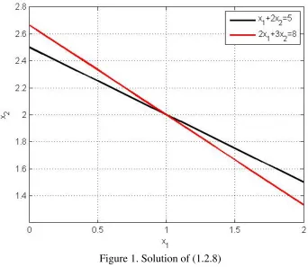
Example 1.2.1: For M N 2, the system
can be written
1
By substitution into (1.2.8), one can easily confirm that
1
is the solution. In this case, the solution can be written in the form (1.2.6) with
1 3 2
2 1
A
Sec. 1.2 •
Systems of Linear Equations
15In the case where M N 2 and M N 3 the system (1.2.2) can be view as defining the common point of intersection of straight lines in the case M N 2 and planes in the case
3
M N . For example the two straight lines defined by (1.2.7) produce the plot
Figure 1. Solution of (1.2.8)
which displays the solution (1.2.9). One can easily imagine a system withM N 2 where the resulting two lines are parallel and, as a consequence, there is no solution.
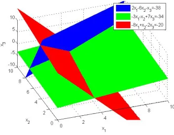
Example 1.2.2: For M N 3, the system
1 2 3
1 2 3
1 2 3
2 6 38
3 7 34
8 2 20
x x x
x x x
x x x
(1.2.11)
defines three planes. If this system has a unique solution then the three planes will intersect in a point. As one can confirm by direct substation, the system (1.2.11) does have a unique solution given by
1 2 3
4 8 2
x x x
The point of intersection (1.2.12) is displayed by plotting the three planes (1.2.11) on a common axis. The result is illustrated by the following figure.
Figure 2. Solution of (1.2.11)
It is perhaps evident that planes associated with three linear algebraic equations can intersect in a point, as with (1.2.11), or as a line or, perhaps, they will not intersect. This geometric observation reveals the fact that systems of linear equations can have unique solutions, solutions that are not unique and no solution. An example where there is not a unique solution is provided by the following:
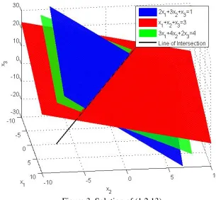
Example 1.2.3:
1 2 3
1 2 3
1 2 3
2 3 1
3
3 4 2 4
x x x
x x x
x x x
(1.2.13)
By direct substitution into (1.2.13) one can establish that
1 3
2 3 3
3 3
8 2 8 2
5 5 5
0 1
x x
x x x
x x
Sec. 1.2 •
Systems of Linear Equations
17obeys (1.2.13) for all values of x3. Thus, there are an infinite number of solutions of (1.2.13). Basically, the system (1.2.13) is one where the planes intersect in a line, the line defined by (1.2.14)3. The following figure displays this fact.
Figure 3. Solution of (1.2.13)
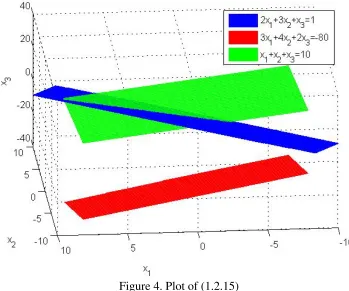
An example for which there is no solution is provided by Example 1.2.4:
1 2 3
1 2 3
1 2 3
2 3 1
3 4 2 80
10
x x x
x x x
x x x
(1.2.15)
Figure 4. Plot of (1.2.15)
A solution does not exist in this case because the three planes do not intersect. Example 1.2.5: Consider the undetermined system
1 2 3
1 2 3
2
2 4
x x x
x x x
(1.2.16)
By direct substitution into (1.2.16) one can establish that
1
2 3
3 3
2
x
x x
x x
x (1.2.17)
is a solution for all values x3. Thus, there are an infinite number of solutions of (1.2.16). Example 1.2.6: Consider the overdetermined system
1 2
1 2
1
2 1 4
x x x x x
Sec. 1.2 •
Systems of Linear Equations
19If (1.2.18)3 is substituted into (1.2.18)1 and (1.2.18)2 the inconsistent results x2 2 and x2 3 are
obtained. Thus, this overdetermined system does not have a solution.
The above six examples illustrate the range of possibilities for the solution of (1.2.3) for various choices of M and N . The graphical arguments used for Examples 1.2.1, 1.2.2, 1.2.3 and 1.2.4 are especially useful when trying to understand the range of possible solutions.
Sec. 1.3 •
Systems of Linear Equations: Gaussian Elimination
21Section 1.3. Systems of Linear Equations: Gaussian Elimination
Elimination methods, which represent methods learned in high school algebra, form the basis for the most powerful methods of solving systems of linear algebraic equations. We begin this discussion by introducing the idea of an equivalent system to the given system (1.2.1). An equivalent system to (1.2.1) is a system of Mlinear algebraic equations in N unknowns obtained from (1.2.1) by
a) switching two rows,
b) multiplying one of the rows by a nonzero constant
c) multiply one row by a nonzero constant and adding it to another row, or d) combinations of a),b) and c).
Equivalent systems have the same solution as the original system. The point that is embedded in this concept is that given the problem of solving (1.2.1), one can convert it to an equivalent system which will be easier to solve. Virtually all of the solution techniques utilized for large systems involve this kind of approach.
Given the system of Mlinear algebraic equations in N unknowns (1.2.1), repeated,
11 1 12 2 13 3 1 1
21 1 22 2 23 3 2 2
1 1 2 2 3 3
N N
N N
M M M MN N M
A x A x A x A x b
A x A x A x A x b
A x A x A x A x b
(1.3.1)
the elimination method consists of the following steps:
Solve the first equation for one of the unknowns, say,x1 if A11 0
Substitute the result into the remaining M 1 equations to obtain M 1 equations in N 1 unknowns, x x2, 3,...,xN.
Repeat the process with these M 1equations to obtain an equation for one of the unknowns.
This solution is then back substituted into the previous equations to obtain the answers for the other two variables.
If the original system of equations does not have a solution, the elimination process will yield an
Example 1.3.1: Given achieved if we multiple the first equation by 2 and subtract it from the second. The result is
1 2 3
elimination method utilizes these two equations to eliminate x2. This elimination is achieved if we multiply (1.3.4)2 by
Step 4: The next step starts a back substitution process. First, we recognize that (1.3.5)3 yields
3 2
x (1.3.6)
This result is substituted into (1.3.5)2 to yield
Sec. 1.3 •
Systems of Linear Equations: Gaussian Elimination
23Step 5: We continue the back substitution process and use (1.3.6) and (1.3.8) to derive from (1.3.5)1
1 1
x (1.3.9)
Therefore, the solution is
1
It should be evident that the above steps are not unique. We could have reached the same endpoint with a different sequence of rearrangements. Also, it should be evident that one could generalize the above process to very large systems.
Example 1.3.2:
We shall use Gaussian elimination to show that
1
Unlike the last example, we shall not directly manipulate the actual equations (1.3.11). We shall simply do matrix manipulations on the coefficients. This is done by first writing the system (1.3.11) as a matrix equation. The result is
1
The next formal step is to form what is called the augmented matrix. It is simply the matrix 1 3 1
augmented by the column matrix 1
. It is customarily given the notation
12 31 1 11 5Next, we shall do the Gaussian elimination procedure directly on the augmented matrix.
Step 1: Multiply the first row by 2 (the A21 element), divide it by 1 (the A11 element) and subtract the first row from the second. The result is
2 row 1
Repeating this process, which is called pivoting,
2 row 1
The last augmented matrix coincides with the system
1 2 3
The next step starts the back substitution part of the process. Equation (1.3.17)3 yields
3 2
x (1.3.18)
Sec. 1.3 •
Systems of Linear Equations: Gaussian Elimination
25Therefore, we have found the result (1.3.12)
The above steps can be generalized without difficulty. For simplicity, we shall give the generalization for the case where M N. The other cases will eventually be discussed but the details can get too involved if we allow those cases at this point in our discussions. For a system of
N equations and N unknowns, we have the equivalence between the system of equations (1.3.1) and its representation by the augmented matrix as follows:
We then, as the above example illustrate, can perform the operations on the rows of the augmented matrix, rather than on the equations themselves.
Note: In matrix algebra, we are using what is known as row operations when we manipulate the augmented matrix.
Step 1: Forward Elimination of Unknowns:
If A11 0, we first multiply the row of the augmented matrix equation by 21 11
A
A and subtract
11 12 13 1 1
In order to keep the notation from becoming unwieldy, we shall assign different symbols to the second row and write (1.3.21) as
Next, we repeat the last procedure for the third row by multiply the first row by 31 11
A
A and subtract
the result from the third equation. The result can be written
Sec. 1.3 •
Systems of Linear Equations: Gaussian Elimination
27The augmented result (1.3.24) corresponds to the system of equations The result is that the original N equations are replaced by
coefficient or pivotelement.
The next step is to apply the same process to the set of N 1 equations with N 1
to eliminate the second unknown, x2. This process begins by multiplying the second row of
(1.3.24) by
You should now have the idea. You continue this process until the augmented matrix (1.3.20)2 is replaced by the upper triangular form
Each step in the process leading to (1.3.28) has assumed we have not encountered the situation where the lead coefficient in the pivot row was zero. The augmented matrix (1.3.28) corresponds to the system of equations
Step 2: Back Substitution
Sec. 1.3 •
Systems of Linear Equations: Gaussian Elimination
29 The formula for these unknowns, should it ever prove useful, is( 1) ( 1)
The process just described make repeated use of the assumption that certain coefficients were nonzero in order for the process to proceed. If one cannot find a coefficient with this property, then the system is degenerate in some way and may not have a unique solution or any solution. Frequently one avoids this problem by utilizing a procedure by what is called partial pivoting. The following example illustrates this procedure.
Example 1.3.3: Consider the system of equations
2 3
The procedure we described above would first create the auxiliary matrix representation of this system. The result is
Because A11 0, we immediately encounter a problem with our method. The partial pivoting procedure simply reorders the equations such that the new A11 0. For example, we can begin the elimination process with the auxiliary matrix
42 63 6 57 3The usual practice is to switch the order of the equations so as to make the A11 the largest, in absolute value, of the elements in the first column.
1 2 3
This system has the solution (1.2.14), repeated,
1 3
It is helpful to utilize the Gauss Elimination procedure to see this solution. The first step is to form the augmented matrix
21 13 1 11 3The sequence of steps described above, applied to this example, is
1
Sec. 1.3 •
Systems of Linear Equations: Gaussian Elimination
31The last augmented matrix coincides with the system
1 2 3
The occurrence of the row of zeros in the third row, results in only two equations for the three unknowns x x1, 2 and x3. The next step starts the back substitution part of the process. Equation (1.3.40)2 yields
2 3 5
x x (1.3.41)
Therefore, from equation (1.3.40)1,
Therefore, we have found the result (1.3.36)
Example 1.3.5: In Section 1.2 we discussed Example 1.2.4 which was the system
It was explained in Section 1.2 that this system does not have a solution. This conclusion arises from the Gauss Elimination procedure by the following steps. As usual, the first step is to form the augmented matrix
The sequence of steps described above, applied to this example, is
3
Repeating this process,
3
The last augmented matrix coincides with the system
Sec. 1.3 •
Systems of Linear Equations: Gaussian Elimination
33Of course, the last equation is inconsistent. The only conclusion is that there is no solution to the system (1.3.43). This is the analytical conclusion that is reflective of the graphical solution attempted with Figure 4 of Section 1.2.
Example 1.3.6: All of examples in this section are examples where M N 3. The assumption
M N was made when we went through the detailed development of the Gauss elimination process. The method also works for cases where the number of equations and the number of unknowns are not the same. The following undetermined system is an illustration of this case.
1 2 3 4 5
As usual, the first step is to form the augmented matrix
14 25 104 6 18 43 9 1The sequence of steps that implement the Gauss elimination is
Subtract 4 row1 from row2
Subtract 7 row1 Subtract 2 row2
from row3 from row3
1 2 4 3 9 1 1 2 4 3 9 1
The last augmented matrix coincides with the system
1 2 3 4 5
The back substitution process takes the third equation of the set (1.3.51) and eliminates x4 or x5
1
The Gauss elimination process applied to the augmented matrix produces attempts to produce a triangular form as illustrated with (1.3.28). Example 1.3.2, which involved a system (1.3.11) that had a unique solution produced a final augmented matrix of the form (see equation (1.3.16))
Example 1.3.4, which involved a system (1.3.35) that did not have a unique solution produced a final augmented matrix of the form (see equation (1.3.39))
2 3 1 1
Example 1.3.5, which involved a system (1.3.43) that did not have a solution produced a final augmented matrix of the form (see equation (1.3.46))
2 3 1 1
Our last example, Example 1.3.6, which involved an undetermined system (1.3.51) produced a final augmented matrix of the form (see equation (1.3.50))
1 2 4 3 9 1
Sec. 1.3 •
Systems of Linear Equations: Gaussian Elimination
35regardless of where it ends, is known as the row echelon form. This upper triangular matrix can be given a more formal definition as follows:
Definition: A MN matrix A is in is in row echelon form if
1) Rows with at least one nonzero element are above any rows of all zero.
2) The first nonzero element from the left (the pivot element) of a nonzero row is always strictly to the right of the leading coefficient of the row above it.
3) The leading coefficient of each nonzero row is 1 .
The above examples, with minor rearrangement in the first three cases, are row echelon matrices. The minor rearrangement involve insuring 3) is obeyed by simply normalizing the row by division. It should be evident that the results are
The row echelon form is one step away from another upper triangular matrix we shall identify in later sections called a reduced row echelon form. These concepts, which are important, will be discussed in the following sections of this chapter.
Exercises
1.3.1 Complete the solution of (1.3.32). The answer is
Sec. 1.3 •
Systems of Linear Equations: Gaussian Elimination
371.3.4 Solve the system
1 2 3 4 5
1 2 5
1 2 5
3 4 5
1 2 3 4 5
1 1
2 2 3 1
3 1
2 2 4 1
x x x x x
x x x
x x x
x x x
x x x x x
(1.3.64)
Sec. 1.4 • Elementary Row Operations, Elementary Matrices 39
Section 1.4. Elementary Row Operations, Elementary Matrices
The last section illustrated the Gauss method of elimination for finding the solution to systems of linear equations. The basic method that is implemented with the method is to perform row operations that are designed to build a row echelon matrix at the end of the process. If the system allows it, one builds an upper triangular matrix that allows the solution to be found by back substitution. As summarized at the start of Section 1.3, the row operations are simply creating equivalent systems of linear equations that, at the end of the process, are easier to solve than the original equations. The row operations utilized in the Gauss elimination method are
a) switching two rows,
b) multiplying one of the rows by a nonzero constant
c) multiply one row by a nonzero constant and adding it to another row, or d) combinations of a),b) and c).
The first three of these row operations are call elementary row operations. They are the building blocks for the fourth operation. It is useful for theoretical and other purposes to implement the elementary row operations by a matrix multiplication operation utilizing so called elementary matrices.
Elementary matrices are square matrices. We shall introduce these matrices in the special case of a system of M 3 equations in N 4 unknowns. The generalization to different size
If we wish to implement a row operation, for example, that switches the first and second row, we can form the product
11 12 13 14 1
11 12 13 14 1
The result of the multiplication is the original augmented matrix except that its first two rows are
switched. The matrix that achieved this row operation,
0 1 0
, is an example of an elementary
matrix. Note that the elementary matrix that switches rows is no more than the identity matrix with its two rows switched. This is a general property of elementary matrices. If we were wished to multiply the second row of
Ab by a constant, say , we would multiply it by the matrix. If we wish to define an elementary matrix that adds the second row to the and third
row of a matrix we would multiply
Ab by the matrixoperations can be implemented by multiplications by elementary matrices. Example 1.4.1: In Example 1.3.3, we looked at the system (1.3.35), repeated,
1 2 3
Sec. 1.4 • Elementary Row Operations, Elementary Matrices 41
The final step in creating the row echelon form from
2 3 1 1
is to normalize the first row
by a division by 2 and the second row by a division by 1 2
Divide row 2
From a computational standpoint, the method of solution utilized in Section 1.3 is preferred. It achieves the final row echelon form without the necessity of identifying the elementary matrices. However, as indicated above, it is a useful theoretical result that
A MN matrix A can be converted to a MN matrix in row echelon form by multiplication of A by a finite number of MM elementary matrices.
Equation (1.4.6) illustrates this assertion in the particular case where the matrix A is an augmented matrix associated with finding the solution of a system of M N equations.
Example 1.4.2: In Example 1.3.6, we looked at the system (1.3.48), repeated,
1 2 3 4 5
Sec. 1.4 • Elementary Row Operations, Elementary Matrices 43
Subtract 7 row1 Subtract 4 row1 Given augmented matrix from row3 from row2
1 0 0 1 0 0 1 2 4 3 9 1
1.4.1 Find the row echelon form of the matrix
Express the result in terms of elementary matrices. 1.4.2 Find the row echelon form of the matrix
Express the result in terms of elementary matrices 1.4.3 Find the row echelon form of the matrix
Sec. 1.5 • Gauss-Jordan Elimination, Reduced Row Echelon Form 45
Section 1.5. Gauss-Jordan Elimination, Reduced Row Echelon Form
In Section 1.3, we introduced the Gauss elimination method and identified the row echelon form as the final form of the elimination method that one reaches by the method. In this section, we shall extend the method by what is known as the Gauss-Jordan elimination method and identify the so called reduced row echelon form of the augmented matrix.
We shall continue to discuss the problem that led to (1.3.28), namely, a system of M N
equations and N unknowns. Equation (1.3.28), repeated, is
In order to reach this result, we have assumed that the pivot process did not yield zeros as the lead element in any row. If this had been the case, the elimination scheme would have not reached the triangular form shown in (1.5.1). The next step in the Gauss elimination method is to utilize back substitution to find the solution. The Gauss-Jordan elimination scheme is a refinement of the Gauss elimination method. It avoids back substitution by implementing additional row operations which zero the elements in the upper triangular part of the matrix. This scheme is best illustrated by an example.
Example 1.5.1: In Section 1.3, we worked Example 1.3.2. This example involved finding the solution of
The augmented matrix is given by (1.3.14) and the row echelon form, which in this case, was an upper triangular matrix is given by (1.3.57). This row echelon form is
The Gauss-Jordan process begins with (1.5.3) and proceeds as follows
1 Subtract row 3
Subtract row 3
from row 1 5
from row 2
Subtract 3 row 2 from row 1
The final matrix in (1.5.4) shows that the solution is
1
which is the result (1.3.12). The matrix
1 0 0 2
Jordan elimination process, is the reduced row echelon matrix in this example.
Example 1.5.2: In Section 1.3, we considered Example 1.3.3. The augmented matrix in this example is given by (1.3.34), repeated,
42 63 6 57 3Sec. 1.5 • Gauss-Jordan Elimination, Reduced Row Echelon Form 47
The Gauss-Jordan portion of the solution picks up from (1.5.7) with the steps
5 Add row 3
12 to row 2
Subtract 7 row 3 Subtract 6 row 2
from row 1 from row 1
1
The Gauss-Jordan elimination method illustrated above is easily applied to cases of
underdetermined systems and overdetermined systems. The following illustrates the method for an underdetermined system.
Example 1.5.3: In Section 1.3, we considered Example 1.3.6. We looked at the same example in Section 1.4 when we worked Example 1.4.2. The end of the Gauss elimination process produced the augmented matrix(1.3.60), repeated,
1 2 4 3 9 1
The special form of (1.5.10) makes the Gauss-Jordan part of the elimination simply from a numerical standpoint. Consider the following steps
2 row 3 subtracted from row 2
3 row 3 2 row 2
subtracted from subtracted from
row 1 row 1
The final result, which is in reduced row echelon form, displays the solution (1.3.52), repeated,
1
The reduced row echelon matrix, that is determined after completion of the Gauss-Jordan elimination method, is defined formally as follows:
Sec. 1.5 • Gauss-Jordan Elimination, Reduced Row Echelon Form 49
2) The first nonzero element from the left (the pivot element) of a nonzero row is always strictly to the right of the leading coefficient of the row above it.
3) The leading coefficient of each nonzero row is 1 and is the only nonzero entry in its column.
If this definition is compared to that of the row echelon form of a matrix given in Section 1.3, then a reduced row echelon form of a matrix is a row echelon form with the property that the entries above and below the leading coefficient are all zero. In Section 1.4 it was explained how the row echelon form of a matrix can be found by a series of multiplications by elementary matrices. If the additional row operations that implement the Gauss-Jordan elimination are represented by
multiplications by row operations, we have the equivalent result
A MN matrix A can be converted to a MN matrix in reduced row echelon form by multiplication of A by a finite number of MM elementary matrices.
Exercises:
1.5.1 Use row operations to find the reduced row echelon form of the matrix
This augmented matrix arose earlier in Exercise 1.3.2. The answer is
1 0 0 0 4
1.5.2 Use row operations to find the reduced row echelon form of the matrix
11 23 13 42 64
This augmented matrix arose in Exercise 1.3.3. The answer is
1 0 0 0 2
1.5.4 Use row operations to find the reduced row echelon form of the matrix
This augmented matrix arose in Exercise 1.3.4. The answer is
1 0 0 0 0 0
1.5.5 Find the solution or solutions of the following system of equations
1 2 3
1.5.6: Find the solution or solutions of the following system of equations
1 2 3
Sec. 1.5 • Gauss-Jordan Elimination, Reduced Row Echelon Form 51
1 2 3 4
1 2 3 4
1 2 3 4
2 3 4 6
3 2 4
2 5 2 5 10
x x x x
x x x x
x x x x
Sec. 1.6 • Elementary Matrices-More Properties 53
Section 1.6. Elementary Matrices-More Properties
In this section we shall look deeper into the idea of an elementary matrix. This concept was introduced in Section 1.4. In that section, we explained that an elementary matrix is a MM
matrix that when it multiplies a MN matrix A will achieve one of the following operations on
A:
a) switch two rows,
b) multiply one of the rows by a nonzero constant,
c) multiply one row by a nonzero constant and add it to another row.
The objective of the elementary matrices is to cause row operations which can transform a matrix, first, into its row echelon form and, second, to its reduced row echelon form. In Sections 1.4 and Sections 1.5, this fact was summarized with the statement
A MN matrix A can be converted to a MN in row echelon form and its reduced row echelon form by multiplication of A by a finite number of MM
elementary matrices.
The row echelon form as the result of multiplication by elementary matrices was illustrated with examples in Section 1.4. The additional multiplications by elementary matrices that convert a matrix from its row echelon form to its reduced row echelon form are illustrated by the following example.
Example 1.6.1: Example 1.4.2, which originated from a desire to solve the system of equations,
1 2 3 4 5
1 2 3 4 5
1 2 3
2 4 3 9 1
4 5 10 6 18 4
7 8 16 7
x x x x x
x x x x x
x x x
(1.6.1)
Subtract 2 row2
Subtract 7 row1 Subtract 4 row1 Given augmented matrix from row3 from row2
1 0 0 1 0 0 1 2 4 3 9 1
The problem is to find the elementary matrices that will convert the matrix
Row echelon form into is reduced row echelon form. As explained in Section 1.4, the elementary matrices are derived from the identity matrix by applying the desired row operation to the identity matrix. The three row operations that achieve this step are shown in equation (1.5.11). Therefore the elementary matrices that achieve these steps are as follows:
1) 2 row 3 subtracted from row 2
2 row 3 subtracted from row 2
3 row 3 subtracted from row 1
2 row 2 subtracted from row 1
Sec. 1.6 • Elementary Matrices-More Properties 55
2 row 2 subtracted 3 row 3 subtracted 2 row 3 subtracted from row 1 from row 1 from row 2
reduced row echelon form from row echelon form
Subtract 2 row2
Subtract 7 row1 Subtract 4 row1 Given augmented matrix
ow3 from row3 from row2
Calculates row echelon form
1 0 0 1 0 0 1 2 4 3 9 1
It is a property of elementary matrices that they are nonsingular. We shall illustrate this assertion by consideration of three examples.
Example 1.6.2: If you are given the elementary matrix that corresponds to switching the first and second row, i.e.,
Example 1.6.3: If you are given the elementary matrix that corresponds to multiplying the second row by a nonzero constant, i.e.,
2
can be substituted into (1.6.11) and verify that it is the inverse. Just as (1.6.10) corresponds to multiplying the second row by the nonzero constant , its inverse, (1.6.12), corresponds to dividing the second row by the nonzero constant .
Example 1.6.4: If you are given the elementary matrix that corresponds to multiplying the third row by a constant and adding the result to the first, i.e.,
Sec. 1.6 • Elementary Matrices-More Properties 57
can be substituted into (1.6.14) and verify that it is the inverse. Just as (1.6.13) corresponds to multiplying the third row by a nonzero constant and adding the result to the first, (1.6.15)
corresponds to multiplying the third row by a nonzero constant and subtracting the result from the first row.
In summary, we have the following two facts about elementary matrices:
1) An elementary matrix is a MM matrix obtained from the M M identity matrix by an elementary row operation.
2) If E is an elementary matrix, then E is nonsingular and, its inverse, E1 is an elementary matrix of the same type.
Definition: A MN matrix B is row equivalent to a M N matrix A if there exist a finite number of elementary matrices E E1, 2,...,Ek such that
2 1
k
BE E E A (1.6.16)
This definition is an adoption of the idea of equivalence to matrices which we introduced in Section 1.3 for systems of equations. It is possible to use the definition (1.6.16) to establish the following two important properties of row equivalence:
1) If B is equivalent to A, then A is equivalent to B.
2) If B is equivalent to A and A equivalent to C, then B is equivalent to C. The proof of the first property follows directly from the definition (1.6.16). The details are as follows. Because each elementary matrix is nonsingular, we can repeatedly use the identity (1.1.36) and establish from (1.6.16) that
If we are given that A is a square matrix, we can identify three properties of A that relate to whether or not it is nonsingular.
Theorem 1.6.1: The following three conditions are equivalent for a square matrix A. a) A is nonsingular.
b) The equation Ax0 only has the solution x0. c) A is row equivalent to the identity matrix I.
Proof: The proof requires that we accept any one of the propositions as true and, from that proposition, prove that the other two are also true. We begin by accepting a) and showing that a) implies b).
a)b): If Ais nonsingular, the equation Ax0 can be multiplied by its inverse to obtain
1
A A xIx x 0. Thus b) is established. Given b), we shall next show that it implies c).
b)c): We are given that the system Ax0 only has the solution x0. Let E E1, 2,...,Ek
be elementary matrices selected such that
2 1
k
U E E E A (1.6.18)
is in reduced row echelon form. It follows from Ax0 and (1.6.18) that
2 1
k
UxE E E Ax0
Because x0 is the only solution allowed by the equation Ux0, the matrix Ucannot have a zero on its diagonal. If it did, for example, in the NN position, this would allow xN 0 which would violate the condition that x0. Because the reduced row echelon form of the matrix which has nonzero diagonal elements has the identity I for its reduced row echelon form, the result is established.
Given c), we shall next show that it implies a).
c) a): We are given that A is row equivalent to the identity matrix I . Therefore, there exists elementary matrices E E1, 2,...,Ek such that
2 1
k
I E E E A (1.6.19)
Sec. 1.6 • Elementary Matrices-More Properties 59
where we have again used the identity (1.1.36). Equation (1.6.21) establishes that A is nonsingular.
It is a corollary to the last result that the system of N equations with N unknowns Axb has a unique solution if and only if A is nonsingular. The argument to prove this corollary is as follows: First, assume the square matrix A is nonsingular, it then follows from Axb that the solution exists and is uniquely given by xA1b. Conversely, we need to prove that if only unique solutions exist, the square matrix A must be nonsingular. The proof of this part of the corollary, like virtually all uniqueness proofs, begins with the assumption that the solution is not unique and then establishes condition that will force uniqueness. We begin with the assumption that there exist two solutions, x1 and x2, that obey
Given (1.6.22) and (1.6.23), it is true that
1 2
1A x x Ax Ax2 b b 0 (1.6.24)
Equation (1.6.24) and part b) of Theorem 1.6.1 tell us that x1x2 0 if and only if A is nonsingular,
Theorem 1.6.1 tells us that in those cases where A is nonsingular we can construct the inverse A1 by finding the elementary matrices E E1, 2,...,Ek which satisfy (1.6.19). When these elementary matrices are known, we can calculate A1 from (1.6.21).
1 3 1
which is the coefficient matrix in Example 1.3.2. This is also the matrix utilized in Example 1.5.1. Consider the following sequence of elementary matrices:
Sec. 1.6 • Elementary Matrices-More Properties 61
Subtract 3 row 2 from row 1
8 6 5
If the multiplications shown in (1.6.34) are carried out, the result is
1
Example 1.6.6: As an additional example, consider the following matrix A and the following sequence of elementary matrices:
Sec. 1.6 • Elementary Matrices-More Properties 63
Multiply row 3 by -1
Step 7
7 6 5 4 3 2 1
Sec. 1.6 • Elementary Matrices-More Properties 65
If this multiplication is performed, the following result is obtained for A1
1
The above two examples illustrates how the elementary matrices generate the inverse for a nonsingular matrix. These examples are illustrations of the theoretical formula (1.6.21). As a practical matter, we are typically only interested in the inverse and not the recording of the individual elementary matrices. A computational algorithm based upon the augmented matrix approach gives the answer more directly. We shall illustrate this algorithm for the matrix in the second example above, i.e. the matrix defined by (1.6.36). The procedure is as follows:
First, form the augmented matrix
A I :We next perform row operations on this auxiliary matrix until an identity appears in the left slot. The step by step process is the following:
Step 3(Multiply row 2 by 1/2.)
Step 5:(Subtract row 2 from row 3)
Sec. 1.6 • Elementary Matrices-More Properties 67
Step 7:(Multiply row 2 by 4 and subtract from row 1.)
7 6 5 4 3 2 1
If the matrix A is singular, the above calculation process will not reduce to the identity matrix in the left slot. In the singular case, of course, the formula (1.6.21), i.e., 1
1 3 3
A as the product of a finite number of elementary matrices.
1.6.2 Use the computational algorithm illustrated above to determine the inverse of 2 1 0
Sec. 1.7 • LU Decomposition
69
Section 1.7.
LUDecomposition
At this point in our understanding of Matrix Algebra, we have two closely related approaches for solving systems of linear algebraic equations. One is based upon Gauss
Elimination, and the other method is based upon Gauss-Jordan Elimination. There is another class of solution methods based upon decompositions of the matrixA. Decomposition is the ability to start with an M N matrixA, and derive from A two or more matrices which allow A to be decomposed into the product
1 2 k
A A A A (1.7.1)
The fact that methods of this type exist is that the factors in the decomposition have properties which make the subsequent solution of
Axb (1.7.2)
easier. One such method is called the LU Decomposition. It is the assertion, which we shall prove, that the A can be decomposed in the form
ALU (1.7.3)
where
U An upper triangle MN matrix and
L A lower triangle nonsingular MM matrix with 1’s down the diagonal.
Example 1.7.1: If A is the matrix we have used before 2 4 2 1 5 2 4 1 9
A
(1.7.4)
1 0 0
In this section, we shall see how to perform the decomposition in general and show how results like (1.7.5) are obtained.
The example (1.7.5) shows that LU Decompositions do exist. However, one of the many questions about this decomposition is whether or not they always exist. If it does not always exist for everyMN matrix, then can we characterize those situations when it does? The answer is that it does not always exist. However, while it cannot be discussed here, it is true that a minor
generalization of this decomposition always exists.3 It turns out that the factorization (1.7.3) always exists if the following is true:
If the MN matrix A can be reduced to upper triangular form without using partial pivoting (i.e. row switching) then A has an LU decomposition.
We shall give an example below where the LU decomposition does not exist. For the moment, we shall proceed and see what problems arises as we attempt the construction.
The reason the LU decomposition is useful is that it allows the equation Axb to be written
LUxb (1.7.6)
Because L, is nonsingular, we can multiply on the left by 1
L and obtain
1 1
L LU xIUxUxLb (1.7.7)
Because U is an upper triangular matrix, the equation
1
UxLb (1.7.8)
can be solved, for example, by back substitution or Gauss-Jordan elimination. Another benefit of the LUDecomposition, and perhaps the most significant benefit, is that it depends only on the properties of A. In other words, the decomposition does not depend upon b. This means that we can perform the decomposition and then solve for x for a variety of choices of b. The methods we have used to date, Gauss Elimination and Gauss-Jordan Elimination, involved manipulations of
3
Sec. 1.7 • LU Decomposition
71
the augmented matrix,
Ab , and, as a consequence, the intermediate calculations depended upon the specific b.The source of the method to create the LU Decomposition is actually Gauss Elimination. When the decomposition can be achieved, Gauss Elimination will give us the matrix U . Our challenge is to discover how to find L such that ALU. The construction of U begins with certain row operations on A. As these operations are conducted, either with elementary matrices or by row operations, we shall see that we build the matrix L.
As a motivation of how Gauss Elimination plays a role in the derivation of ALU, it is instructive to try what is essentially a brute force method. We shall briefly illustrate this method in the case where A is a 3 3 matrix. In this case, the equation we hope to derive, namely (1.7.3), can be written in components as
11 12 13 11 12 13
Equation (1.7.9) connects the given nine components of A on the left side to the unknown three components of L and the six components of U on the right side. If we evaluate the product on the right hand side, the result is
11 12 13 11 12 13
Our goal is to calculate the nine unknown quantities that appear on the right side of (1.7.10). Equating like elements on both sides of (1.7.10), the first row yields
11 11
If we assume A11 0, then the three unknowns in (1.7.12) are given by
The three equations from the third row are
31 31 11 31 11
32 31 12 32 22 31 12 32 22
31 32 33
33 31 13 32 23 33 31 13 32 23 33
3 Eqs and 3 Unknowns ( , and ) use these formulas to produce the result (1.7.5) shown in Example 1.7.1. This derivation also shows that not all matrices have a LU decomposition like (1.7.3). An example where the above formulas cannot be used is the following:
Example 1.7.2:
Because of the two zeros in the second column of the matrix (1.7.16), (1.7.13)3 shows that U22 0
Sec. 1.7 • LU Decomposition
73
In those cases where (1.7.13) and (1.7.15) are valid, it should be noted that the steps
dictated by the above formulas implement the following rearrangements to
11 12 13
This result shows that the second row of U is simply the second row of the matrix equivalent to A
obtained by Gauss elimination. If one studies the above formulas one can also conclude that the third row is also what one would obtain by Gauss elimination. These facts reveal an alternate way of generating the LU Decomposition.
Recall that we implemented Gauss Elimination by performing row operations. a) switching two rows,
b) multiplying one of the rows by a nonzero constant
c) multiply one row by a nonzero constant and adding it to another row.
We mainly used c). The operation b) was used when we chose to normalize a row such as occurs when finding the row echelon form of a matrix. The operation a) was used when the occurrence of a zero made it necessary to change the pivot row. An important fact is that the method of finding building the LU Decomposition will only make use of c). It will not proceed with row operations that produce the row echelon form or the reduced row echelon. It will proceed to the point where the coefficient matrix is an upper triangular form as with the Gauss Elimination examples discussed in Section 1.3. Of course, we can view these row operations in the equivalent way as elementary matrix operations.
The key to finding the matrix L with the specified properties is to simply set up a tracking system as the matrix U is derived. The key to the tracking system is equation (1.7.8). It is a feature of the calculation that we shall actually construct 1
L . After it is calculated, it can be inverted to yield the L in the decomposition ALU.