▸ Baca selengkapnya: c++ how to program (10th edition) pdf
(2)The most important systems of units are shown in the table below. The mks system is also known as the International System of Units (abbreviated SI), and the abbreviations sec (instead of s), gm (instead of g), and nt (instead of N) are also used.
System of units Length Mass Time Force
cgs system centimeter (cm) gram (g) second (s) dyne
mks system meter (m) kilogram (kg) second (s) newton (nt)
Engineering system foot (ft) slug second (s) pound (lb)
1 inch (in.) ⫽2.540000 cm 1 foot (ft) ⫽12 in. ⫽30.480000 cm
1 yard (yd) ⫽3 ft ⫽91.440000 cm 1 statute mile (mi) ⫽5280 ft ⫽ 1.609344 km 1 nautical mile ⫽ 6080 ft ⫽1.853184 km
1 acre ⫽4840 yd2
⫽4046.8564 m2 1 mi2
⫽640 acres ⫽2.5899881 km2 1 fluid ounce ⫽ 1/128 U.S. gallon ⫽231/128 in.3
⫽29.573730 cm3 1 U.S. gallon ⫽ 4 quarts (liq) ⫽8 pints (liq) ⫽ 128 fl oz ⫽ 3785.4118 cm3 1 British Imperial and Canadian gallon ⫽1.200949 U.S. gallons ⫽4546.087 cm3 1 slug ⫽14.59390 kg
1 pound (lb) ⫽ 4.448444 nt 1 newton (nt) ⫽105dynes
1 British thermal unit (Btu) ⫽1054.35 joules 1 joule ⫽107ergs 1 calorie (cal) ⫽4.1840 joules
1 kilowatt-hour (kWh) ⫽3414.4 Btu ⫽3.6•106joules
1 horsepower (hp) ⫽2542.48 Btu/h ⫽178.298 cal/sec ⫽0.74570 kW 1 kilowatt (kW) ⫽1000 watts ⫽ 3414.43 Btu/h ⫽238.662 cal/s
°F ⫽°C•1.8 ⫹32 1°⫽60
⬘
⫽3600⬙
⫽0.017453293 radianADVANCED
10
T H E D I T I O N
ADVANCED
ENGINEERING
MATHEMATICS
ERWIN KREYSZIG
Professor of Mathematics
Ohio State University
Columbus, Ohio
In collaboration with
HERBERT KREYSZIG
New York, New York
EDWARD J. NORMINTON
Associate Professor of Mathematics
Carleton University
Ottawa, Ontario
MARKETING MANAGER Jonathan Cottrell CONTENT MANAGER Lucille Buonocore PRODUCTION EDITOR Barbara Russiello
MEDIA EDITOR Melissa Edwards
MEDIA PRODUCTION SPECIALIST Lisa Sabatini TEXT AND COVER DESIGN Madelyn Lesure
PHOTO RESEARCHER Sheena Goldstein
COVER PHOTO © Denis Jr. Tangney/iStockphoto
Cover photo shows the Zakim Bunker Hill Memorial Bridge in Boston, MA.
This book was set in Times Roman. The book was composed by PreMedia Global, and printed and bound by RR Donnelley & Sons Company, Jefferson City, MO. The cover was printed by RR Donnelley & Sons Company, Jefferson City, MO.
This book is printed on acid free paper.
Founded in 1807, John Wiley & Sons, Inc. has been a valued source of knowledge and understanding for more than 200 years, helping people around the world meet their needs and fulfill their aspirations. Our company is built on a foundation of principles that include responsibility to the communities we serve and where we live and work. In 2008, we launched a Corporate Citizenship Initiative, a global effort to address the environmental, social, economic, and ethical challenges we face in our business. Among the issues we are addressing are carbon impact, paper specifications and procurement, ethical conduct within our business and among our vendors, and community and charitable support. For more information, please visit our website: www.wiley.com/go/citizenship. Copyright © 2011, 2006, 1999 by John Wiley & Sons, Inc. All rights reserved. No part of this publication may be reproduced, stored in a retrieval system, or transmitted in any form or by any means, electronic, mechanical, photocopying, recording, scanning or otherwise, except as permitted under Sections 107 or 108 of the 1976 United States Copyright Act, without either the prior written permission of the Publisher, or authorization through payment of the appropriate per-copy fee to the Copyright Clearance Center, Inc., 222 Rosewood Drive, Danvers, MA 01923 (Web site: www.copyright.com). Requests to the Publisher for permission should be addressed to the Permissions Department, John Wiley & Sons, Inc., 111 River Street, Hoboken, NJ 07030-5774, (201) 748-6011, fax (201) 748-6008, or online at: www.wiley.com/go/permissions.
Evaluation copies are provided to qualified academics and professionals for review purposes only, for use in their courses during the next academic year. These copies are licensed and may not be sold or transferred to a third party. Upon completion of the review period, please return the evaluation copy to Wiley. Return instructions and a free of charge return shipping label are available at: www.wiley.com/go/returnlabel. Outside of the United States, please contact your local representative.
ISBN 978-0-470-45836-5
Printed in the United States of America 10 9 8 7 6 5 4 3 2 1
P R E F A C E
See also
http://www.wiley.com/college/kreyszig
Purpose and Structure of the Book
This book provides a comprehensive, thorough, and up-to-date treatment of engineering mathematics. It is intended to introduce students of engineering, physics, mathematics, computer science, and related fields to those areas of applied mathematics that are most relevant for solving practical problems. A course in elementary calculus is the sole prerequisite. (However, a concise refresher of basic calculus for the student is included on the inside cover and in Appendix 3.)
The subject matter is arranged into seven parts as follows:
A. Ordinary Differential Equations (ODEs)in Chapters 1–6 B. Linear Algebra. Vector Calculus.See Chapters 7–10
C. Fourier Analysis. Partial Differential Equations (PDEs).See Chapters 11 and 12 D. Complex Analysisin Chapters 13–18
E. Numeric Analysisin Chapters 19–21 F. Optimization, Graphsin Chapters 22 and 23 G. Probability, Statisticsin Chapters 24 and 25.
These are followed by five appendices: 1. References, 2. Answers to Odd-Numbered Problems, 3. Auxiliary Materials (see also inside covers of book), 4. Additional Proofs, 5.Table of Functions. This is shown in a block diagram on the next page.
The parts of the book are kept independent. In addition, individual chapters are kept as independent as possible. (If so needed, any prerequisites—to the level of individual sections of prior chapters—are clearly stated at the opening of each chapter.) We give the instructor maximum flexibility in selecting the materialand tailoring it to his or her need. The book has helped to pave the way for the present development of engineering mathematics. This new edition will prepare the student for the current tasks and the future by a modern approach to the areas listed above. We provide the material and learning tools for the students to get a good foundation of engineering mathematics that will help them in their careers and in further studies.
General Features of the Book Include:
• Simplicity of examples to make the book teachable—why choose complicated examples when simple ones are as instructive or even better?
• Independence of parts and blocks of chapters to provide flexibility in tailoring courses to specific needs.
• Self-contained presentation, except for a few clearly marked places where a proof would exceed the level of the book and a reference is given instead.
• Gradual increase in difficulty of material with no jumps or gaps to ensure an enjoyable teaching and learning experience.
• Modern standard notationto help students with other courses, modern books, and journals in mathematics, engineering, statistics, physics, computer science, and others. Furthermore, we designed the book to be a single, self-contained, authoritative, and convenient sourcefor studying and teaching applied mathematics, eliminating the need for time-consuming searches on the Internet or time-consuming trips to the library to get a particular reference book.
GUIDES AND MANUALS
Maple Computer Guide
Mathematica Computer Guide
Student Solutions Manual
and Study Guide
Instructor’s Manual
PART A
Chaps. 1–6
Ordinary Differential Equations (ODEs)
Chaps. 1–4 Basic Material
Chap. 5 Chap. 6
Series Solutions Laplace Transforms
PART B
Chaps. 7–10
Linear Algebra. Vector Calculus
Chap. 7 Chap. 9
Matrices, Vector Differential
Linear Systems Calculus
Chap. 8 Chap. 10
Eigenvalue Problems Vector Integral Calculus
P A R T S A N D C H A P T E R S O F T H E B O O K
PART C
Chaps. 11–12
Fourier Analysis. Partial Differential
Equations (PDEs)
Chap. 11 Fourier Analysis
Chap. 12
Partial Differential Equations
PART D
Chaps. 13–18
Complex Analysis,
Potential Theory
Chaps. 13–17 Basic Material
Chap. 18 Potential Theory
PART E
Chaps. 19–21
Numeric Analysis
Chap. 19 Chap. 20 Chap. 21
Numerics in Numeric Numerics for
General Linear Algebra ODEs and PDEs
PART F
Chaps. 22–23
Optimization, Graphs
Chap. 22 Chap. 23
Linear Programming Graphs, Optimization
PART G
Chaps. 24–25
Probability, Statistics
Chap. 24
Data Analysis. Probability Theory
Four Underlying Themes of the Book
The driving force in engineering mathematics is the rapid growth of technology and the sciences. New areas—often drawing from several disciplines—come into existence. Electric cars, solar energy, wind energy, green manufacturing, nanotechnology, risk management, biotechnology, biomedical engineering, computer vision, robotics, space travel, communication systems, green logistics, transportation systems, financial engineering, economics, and many other areas are advancing rapidly. What does this mean for engineering mathematics? The engineer has to take a problem from any diverse area and be able to model it. This leads to the first of four underlying themes of the book.
1. Modeling is the process in engineering, physics, computer science, biology,
chemistry, environmental science, economics, and other fields whereby a physical situation or some other observation is translated into a mathematical model. This mathematical model could be a system of differential equations, such as in population control (Sec. 4.5), a probabilistic model (Chap. 24), such as in risk management, a linear programming problem (Secs. 22.2–22.4) in minimizing environmental damage due to pollutants, a financial problem of valuing a bond leading to an algebraic equation that has to be solved by Newton’s method (Sec. 19.2), and many others.
The next step is solving the mathematical problem obtained by one of the many techniques covered in Advanced Engineering Mathematics.
The third step is interpreting the mathematical result in physical or other terms to see what it means in practice and any implications.
Finally, we may have to make a decision that may be of an industrial nature or recommend a public policy. For example, the population control model may imply the policy to stop fishing for 3 years. Or the valuation of the bond may lead to a recommendation to buy. The variety is endless, but the underlying mathematics is surprisingly powerful and able to provide advice leading to the achievement of goals toward the betterment of society, for example, by recommending wise policies concerning global warming, better allocation of resources in a manufacturing process, or making statistical decisions (such as in Sec. 25.4 whether a drug is effective in treating a disease).
While we cannot predict what the future holds, we do know that the student has to practice modeling by being given problems from many different applications as is done in this book. We teach modeling from scratch, right in Sec. 1.1, and give many examples in Sec. 1.3, and continue to reinforce the modeling process throughout the book.
2. Judicious use of powerful software for numerics(listed in the beginning of Part E)
and statistics (Part G) is of growing importance. Projects in engineering and industrial companies may involve large problems of modeling very complex systems with hundreds of thousands of equations or even more. They require the use of such software. However, our policy has always been to leave it up to the instructor to determine the degree of use of computers, from none or little use to extensive use. More on this below.
3. The beauty of engineering mathematics. Engineering mathematics relies on
4. To clearly identify the conceptual structure of subject matters.For example, complex analysis (in Part D) is a field that is not monolithic in structure but was formed by three distinct schools of mathematics. Each gave a different approach, which we clearly mark. The first approach is solving complex integrals by Cauchy’s integral formula (Chaps. 13 and 14), the second approach is to use the Laurent series and solve complex integrals by residue integration (Chaps. 15 and 16), and finally we use a geometric approach of conformal mapping to solve boundary value problems (Chaps. 17 and 18). Learning the conceptual structure and terminology of the different areas of engineering mathematics is very important for three reasons:
a. It allows the student to identify a new problem and put it into the right group of problems. The areas of engineering mathematics are growing but most often retain their conceptual structure.
b.The student can absorb new information more rapidlyby being able to fit it into the conceptual structure.
c.Knowledge of the conceptual structure and terminology is also important when using the Internet to search for mathematical information. Since the search proceeds by putting in key words (i.e., terms) into the search engine, the student has to remember the important concepts (or be able to look them up in the book) that identify the application and area of engineering mathematics.
Big Changes in This Edition
Problem Sets Changed
The problem sets have been revised and rebalanced with some problem sets having more problems and some less, reflecting changes in engineering mathematics. There is a greater emphasis on modeling. Now there are also problems on the discrete Fourier transform (in Sec. 11.9).
Series Solutions of ODEs, Special Functions and Fourier Analysis Reorganized Chap. 5, on series solutions of ODEs and special functions, has been shortened. Chap. 11 on Fourier Analysis now contains Sturm–Liouville problems, orthogonal functions, and orthogonal eigenfunction expansions (Secs. 11.5, 11.6), where they fit better conceptually (rather than in Chap. 5), being extensions of Fourier’s idea of using orthogonal functions.
Openings of Parts and Chapters Rewritten As Well As Parts of Sections In order to give the student a better idea of the structure of the material (see Underlying Theme 4 above), we have entirely rewritten the openings of parts and chapters. Furthermore, large parts or individual paragraphs of sections have been rewritten or new sentences inserted into the text. This should give the students a better intuitive understanding of the material (see Theme 3 above), let them draw conclusions on their own, and be able to tackle more advanced material. Overall, we feel that the book has become more detailed and leisurely written.
Student Solutions Manual and Study Guide Enlarged
Upon the explicit request of the users, the answers provided are more detailed and complete. More explanations are given on how to learn the material effectively by pointing out what is most important.
More Historical Footnotes, Some Enlarged
Historical footnotes are there to show the student that many people from different countries working in different professions, such as surveyors, researchers in industry, etc., contributed
to the field of engineering mathematics. It should encourage the students to be creative in their own interests and careers and perhaps also to make contributions to engineering mathematics.
Further Changes and New Features
• Parts of Chap. 1 on first-order ODEs are rewritten. More emphasis on modeling, also new block diagram explaining this concept in Sec. 1.1. Early introduction of Euler’s method in Sec. 1.2 to familiarize student with basic numerics. More examples of separable ODEs in Sec. 1.3.
• For Chap. 2, on second-order ODEs, note the following changes: For ease of reading, the first part of Sec. 2.4, which deals with setting up the mass-spring system, has been rewritten; also some rewriting in Sec. 2.5 on the Euler–Cauchy equation. • Substantially shortened Chap. 5, Series Solutions of ODEs. Special Functions:
combined Secs. 5.1 and 5.2 into one section called “Power Series Method,” shortened material in Sec. 5.4 Bessel’s Equation (of the first kind), removed Sec. 5.7 (Sturm–Liouville Problems) and Sec. 5.8 (Orthogonal Eigenfunction Expansions) and moved material into Chap. 11 (see “Major Changes” above).
• New equivalent definition of basis(Sec. 7.4).
• In Sec. 7.9, completely new part on composition of linear transformationswith two new examples. Also, more detailed explanation of the role of axioms, in connection with the definition of vector space.
• New table of orientation (opening of Chap. 8 “Linear Algebra: Matrix Eigenvalue Problems”) where eigenvalue problems occur in the book. More intuitive explanation of what an eigenvalue is at the begining of Sec. 8.1.
• Better definition of cross product (in vector differential calculus) by properly identifying the degenerate case (in Sec. 9.3).
• Chap. 11 on Fourier Analysis extensively rearranged: Secs. 11.2 and 11.3 combined into one section (Sec. 11.2), old Sec. 11.4 on complex Fourier Series removed and new Secs. 11.5 (Sturm–Liouville Problems) and 11.6 (Orthogonal Series) put in (see “Major Changes” above). New problems (new!) in problem set 11.9 on discrete Fourier transform.
• New section 12.5on modeling heat flow from a body in space by setting up the heat equation. Modeling PDEs is more difficult so we separated the modeling process from the solving process (in Sec. 12.6).
• Introduction to Numericsrewritten for greater clarity and better presentation; new Example 1 on how to round a number. Sec. 19.3 on interpolation shortened by removing the less important central difference formula and giving a reference instead. • Large new footnote with historical details in Sec. 22.3, honoring George Dantzig,
the inventor of the simplex method.
• Traveling salesman problemnow described better as a “difficult” problem, typical of combinatorial optimization (in Sec. 23.2). More careful explanation on how to compute the capacity of a cut set in Sec. 23.6 (Flows on Networks).
data, outliers, and the z-score (Sec. 24.1). Furthermore, new example on encription (Sec. 24.4).
• Lists of softwarefor numerics (Part E) and statistics (Part G) updated.
• References in Appendix 1updated to include new editions and some references to websites.
Use of Computers
The presentation in this book is adaptable to various degrees of use of software, Computer Algebra Systems (CAS’s), or programmable graphic calculators, ranging from no use, very little use, medium use, to intensive use of such technology. The choice of how much computer content the course should have is left up to the instructor, thereby exhibiting our philosophy of maximum flexibility and adaptability. And, no matter what the instructor decides, there will be no gaps or jumps in the text or problem set. Some problems are clearly designed as routine and drill exercises and should be solved by hand (paper and pencil, or typing on your computer). Other problems require more thinking and can also be solved without computers. Then there are problems where the computer can give the student a hand. And finally, the book has CAS projects, CAS problemsand CAS experiments, which do requirea computer, and show its power in solving problems that are difficult or impossible to access otherwise. Here our goal is to combine intelligent computer use with high-quality mathematics. The computer invites visualization, experimentation, and independent discovery work. In summary, the high degree of flexibility of computer use for the book is possible since there are plenty of problems to choose from and the CAS problems can be omitted if desired.
Note that information on software(what is available and where to order it) is at the
beginning of Part E on Numeric Analysis and Part G on Probability and Statistics. Since Mapleand Mathematicaare popular Computer Algebra Systems, there are two computer guides available that are specifically tailored to Advanced Engineering Mathematics: E. Kreyszig and E.J. Norminton, Maple Computer Guide, 10th Editionand Mathematica Computer Guide, 10th Edition.Their use is completely optional as the text in the book is written without the guides in mind.
Suggestions for Courses: A Four-Semester Sequence
The material, when taken in sequence, is suitable for four consecutive semester courses, meeting 3 to 4 hours a week:
1st Semester ODEs (Chaps. 1–5 or 1–6)
2nd Semester Linear Algebra. Vector Analysis (Chaps. 7–10) 3rd Semester Complex Analysis (Chaps. 13–18)
4th Semester Numeric Methods (Chaps. 19–21)
Suggestions for Independent One-Semester Courses
The book is also suitable for various independent one-semester courses meeting 3 hours a week. For instance,
Introduction to ODEs (Chaps. 1–2, 21.1) Laplace Transforms (Chap. 6)
Vector Algebra and Calculus (Chaps. 9–10)
Fourier Series and PDEs (Chaps. 11–12, Secs. 21.4–21.7) Introduction to Complex Analysis (Chaps. 13–17) Numeric Analysis (Chaps. 19, 21)
Numeric Linear Algebra (Chap. 20) Optimization (Chaps. 22–23)
Graphs and Combinatorial Optimization (Chap. 23) Probability and Statistics (Chaps. 24–25)
Acknowledgments
We are indebted to former teachers, colleagues, and students who helped us directly or indirectly in preparing this book, in particular this new edition. We profited greatly from discussions with engineers, physicists, mathematicians, computer scientists, and others, and from their written comments. We would like to mention in particular Professors Y. A. Antipov, R. Belinski, S. L. Campbell, R. Carr, P. L. Chambré, Isabel F. Cruz, Z. Davis, D. Dicker, L. D. Drager, D. Ellis, W. Fox, A. Goriely, R. B. Guenther, J. B. Handley, N. Harbertson, A. Hassen, V. W. Howe, H. Kuhn, K. Millet, J. D. Moore, W. D. Munroe, A. Nadim, B. S. Ng, J. N. Ong, P. J. Pritchard, W. O. Ray, L. F. Shampine, H. L. Smith, Roberto Tamassia, A. L. Villone, H. J. Weiss, A. Wilansky, Neil M. Wigley, and L. Ying; Maria E. and Jorge A. Miranda, JD, all from the United States; Professors Wayne H. Enright, Francis. L. Lemire, James J. Little, David G. Lowe, Gerry McPhail, Theodore S. Norvell, and R. Vaillancourt; Jeff Seiler and David Stanley, all from Canada; and Professor Eugen Eichhorn, Gisela Heckler, Dr. Gunnar Schroeder, and Wiltrud Stiefenhofer from Europe. Furthermore, we would like to thank Professors John B. Donaldson, Bruce C. N. Greenwald, Jonathan L. Gross, Morris B. Holbrook, John R. Kender, and Bernd Schmitt; and Nicholaiv Villalobos, all from Columbia University, New York; as well as Dr. Pearl Chang, Chris Gee, Mike Hale, Joshua Jayasingh, MD, David Kahr, Mike Lee, R. Richard Royce, Elaine Schattner, MD, Raheel Siddiqui, Robert Sullivan, MD, Nancy Veit, and Ana M. Kreyszig, JD, all from New York City. We would also like to gratefully acknowledge the use of facilities at Carleton University, Ottawa, and Columbia University, New York.
Furthermore we wish to thank John Wiley and Sons, in particular Publisher Laurie Rosatone, Editor Shannon Corliss, Production Editor Barbara Russiello, Media Editor Melissa Edwards, Text and Cover Designer Madelyn Lesure, and Photo Editor Sheena Goldstein for their great care and dedication in preparing this edition. In the same vein, we would also like to thank Beatrice Ruberto, copy editor and proofreader, WordCo, for the Index, and Joyce Franzen of PreMedia and those of PreMedia Global who typeset this edition.
Suggestions of many readers worldwide were evaluated in preparing this edition. Further comments and suggestions for improving the book will be gratefully received.
xv
C O N T E N T S
P A R T A
Ordinary Differential Equations (ODEs)
1
CHAPTER 1
First-Order ODEs 2
1.1 Basic Concepts. Modeling 2
1.2 Geometric Meaning of y
⬘
⫽ƒ(x, y). Direction Fields, Euler’s Method 9 1.3 Separable ODEs. Modeling 121.4 Exact ODEs. Integrating Factors 20
1.5 Linear ODEs. Bernoulli Equation. Population Dynamics 27 1.6 Orthogonal Trajectories. Optional 36
1.7 Existence and Uniqueness of Solutions for Initial Value Problems 38
Chapter 1 Review Questions and Problems 43
Summary of Chapter 1 44
CHAPTER 2
Second-Order Linear ODEs 46
2.1 Homogeneous Linear ODEs of Second Order 46
2.2 Homogeneous Linear ODEs with Constant Coefficients 53 2.3 Differential Operators. Optional 60
2.4 Modeling of Free Oscillations of a Mass–Spring System 62 2.5 Euler–Cauchy Equations 71
2.6 Existence and Uniqueness of Solutions. Wronskian 74 2.7 Nonhomogeneous ODEs 79
2.8 Modeling: Forced Oscillations. Resonance 85 2.9 Modeling: Electric Circuits 93
2.10 Solution by Variation of Parameters 99
Chapter 2 Review Questions and Problems 102
Summary of Chapter 2 103
CHAPTER 3
Higher Order Linear ODEs 105
3.1 Homogeneous Linear ODEs 105
3.2 Homogeneous Linear ODEs with Constant Coefficients 111 3.3 Nonhomogeneous Linear ODEs 116
Chapter 3 Review Questions and Problems 122
Summary of Chapter 3 123
CHAPTER 4
Systems of ODEs. Phase Plane. Qualitative Methods 124
4.0 For Reference: Basics of Matrices and Vectors 124
4.1 Systems of ODEs as Models in Engineering Applications 130 4.2 Basic Theory of Systems of ODEs. Wronskian 137
4.3 Constant-Coefficient Systems. Phase Plane Method 140 4.4 Criteria for Critical Points. Stability 148
4.5 Qualitative Methods for Nonlinear Systems 152 4.6 Nonhomogeneous Linear Systems of ODEs 160
Chapter 4 Review Questions and Problems 164
Summary of Chapter 4 165
CHAPTER 5
Series Solutions of ODEs. Special Functions 167
5.1 Power Series Method 167
5.3 Extended Power Series Method: Frobenius Method 180 5.4 Bessel’s Equation. Bessel Functions J(x) 187
5.5 Bessel Functions of the Y(x). General Solution 196 Chapter 5 Review Questions and Problems 200
Summary of Chapter 5 201
CHAPTER 6
Laplace Transforms 203
6.1 Laplace Transform. Linearity. First Shifting Theorem (s-Shifting) 204 6.2 Transforms of Derivatives and Integrals. ODEs 211
6.3 Unit Step Function (Heaviside Function). Second Shifting Theorem (t-Shifting) 217
6.4 Short Impulses. Dirac’s Delta Function. Partial Fractions 225 6.5 Convolution. Integral Equations 232
6.6 Differentiation and Integration of Transforms. ODEs with Variable Coefficients 238 6.7 Systems of ODEs 242
6.8 Laplace Transform: General Formulas 248 6.9 Table of Laplace Transforms 249
Chapter 6 Review Questions and Problems 251
Summary of Chapter 6 253
P A R T B
Linear Algebra. Vector Calculus
255
CHAPTER 7
Linear Algebra: Matrices, Vectors, Determinants.
Linear Systems 256
7.1 Matrices, Vectors: Addition and Scalar Multiplication 257 7.2 Matrix Multiplication 263
7.3 Linear Systems of Equations. Gauss Elimination 272 7.4 Linear Independence. Rank of a Matrix. Vector Space 282 7.5 Solutions of Linear Systems: Existence, Uniqueness 288 7.6 For Reference: Second- and Third-Order Determinants 291 7.7 Determinants. Cramer’s Rule 293
7.8 Inverse of a Matrix. Gauss–Jordan Elimination 301
7.9 Vector Spaces, Inner Product Spaces. Linear Transformations. Optional 309
Chapter 7 Review Questions and Problems 318
Summary of Chapter 7 320
CHAPTER 8
Linear Algebra: Matrix Eigenvalue Problems 322
8.1 The Matrix Eigenvalue Problem.
Determining Eigenvalues and Eigenvectors 323 8.2 Some Applications of Eigenvalue Problems 329
8.3 Symmetric, Skew-Symmetric, and Orthogonal Matrices 334 8.4 Eigenbases. Diagonalization. Quadratic Forms 339
8.5 Complex Matrices and Forms. Optional 346
Chapter 8 Review Questions and Problems 352
CHAPTER 9
Vector Differential Calculus. Grad, Div, Curl 354
9.1 Vectors in 2-Space and 3-Space 3549.2 Inner Product (Dot Product) 361 9.3 Vector Product (Cross Product) 368
9.4 Vector and Scalar Functions and Their Fields. Vector Calculus: Derivatives 375 9.5 Curves. Arc Length. Curvature. Torsion 381
9.6 Calculus Review: Functions of Several Variables. Optional 392 9.7 Gradient of a Scalar Field. Directional Derivative 395
9.8 Divergence of a Vector Field 402 9.9 Curl of a Vector Field 406
Chapter 9 Review Questions and Problems 409
Summary of Chapter 9 410
CHAPTER 10
Vector Integral Calculus. Integral Theorems 413
10.1 Line Integrals 413
10.2 Path Independence of Line Integrals 419
10.3 Calculus Review: Double Integrals. Optional 426 10.4 Green’s Theorem in the Plane 433
10.5 Surfaces for Surface Integrals 439 10.6 Surface Integrals 443
10.7 Triple Integrals. Divergence Theorem of Gauss 452 10.8 Further Applications of the Divergence Theorem 458 10.9 Stokes’s Theorem 463
Chapter 10 Review Questions and Problems 469
Summary of Chapter 10 470
P A R T C
Fourier Analysis. Partial Differential Equations (PDEs)
473
CHAPTER 11
Fourier Analysis 474
11.1 Fourier Series 474
11.2 Arbitrary Period. Even and Odd Functions. Half-Range Expansions 483 11.3 Forced Oscillations 492
11.4 Approximation by Trigonometric Polynomials 495 11.5 Sturm–Liouville Problems. Orthogonal Functions 498 11.6 Orthogonal Series. Generalized Fourier Series 504 11.7 Fourier Integral 510
11.8 Fourier Cosine and Sine Transforms 518
11.9 Fourier Transform. Discrete and Fast Fourier Transforms 522
11.10 Tables of Transforms 534
Chapter 11 Review Questions and Problems 537
Summary of Chapter 11 538
CHAPTER 12
Partial Differential Equations (PDEs) 540
12.1 Basic Concepts of PDEs 540
12.2 Modeling: Vibrating String, Wave Equation 543
12.6 Heat Equation: Solution by Fourier Series.
Steady Two-Dimensional Heat Problems. Dirichlet Problem 558 12.7 Heat Equation: Modeling Very Long Bars.
Solution by Fourier Integrals and Transforms 568
12.8 Modeling: Membrane, Two-Dimensional Wave Equation 575 12.9 Rectangular Membrane. Double Fourier Series 577
12.10 Laplacian in Polar Coordinates. Circular Membrane. Fourier–Bessel Series 585
12.11 Laplace’s Equation in Cylindrical and Spherical Coordinates. Potential 593
12.12 Solution of PDEs by Laplace Transforms 600
Chapter 12 Review Questions and Problems 603
Summary of Chapter 12 604
P A R T D
Complex Analysis
607
CHAPTER 13
Complex Numbers and Functions.
Complex Differentiation 608
13.1 Complex Numbers and Their Geometric Representation 608 13.2 Polar Form of Complex Numbers. Powers and Roots 613 13.3 Derivative. Analytic Function 619
13.4 Cauchy–Riemann Equations. Laplace’s Equation 625 13.5 Exponential Function 630
13.6 Trigonometric and Hyperbolic Functions. Euler’s Formula 633 13.7 Logarithm. General Power. Principal Value 636
Chapter 13 Review Questions and Problems 641
Summary of Chapter 13 641
CHAPTER 14
Complex Integration 643
14.1 Line Integral in the Complex Plane 643 14.2 Cauchy’s Integral Theorem 652 14.3 Cauchy’s Integral Formula 660 14.4 Derivatives of Analytic Functions 664
Chapter 14 Review Questions and Problems 668
Summary of Chapter 14 669
CHAPTER 15
Power Series, Taylor Series 671
15.1 Sequences, Series, Convergence Tests 671 15.2 Power Series 680
15.3 Functions Given by Power Series 685 15.4 Taylor and Maclaurin Series 690 15.5 Uniform Convergence. Optional 698
Chapter 15 Review Questions and Problems 706
Summary of Chapter 15 706
CHAPTER 16
Laurent Series. Residue Integration 708
16.1 Laurent Series 708
16.2 Singularities and Zeros. Infinity 715 16.3 Residue Integration Method 719
16.4 Residue Integration of Real Integrals 725
Chapter 16 Review Questions and Problems 733
CHAPTER 17
Conformal Mapping 736
17.1 Geometry of Analytic Functions: Conformal Mapping 737 17.2 Linear Fractional Transformations (Möbius Transformations) 742 17.3 Special Linear Fractional Transformations 746
17.4 Conformal Mapping by Other Functions 750 17.5 Riemann Surfaces. Optional 754
Chapter 17 Review Questions and Problems 756
Summary of Chapter 17 757
CHAPTER 18
Complex Analysis and Potential Theory 758
18.1 Electrostatic Fields 759
18.2 Use of Conformal Mapping. Modeling 763 18.3 Heat Problems 767
18.4 Fluid Flow 771
18.5 Poisson’s Integral Formula for Potentials 777 18.6 General Properties of Harmonic Functions.
Uniqueness Theorem for the Dirichlet Problem 781
Chapter 18 Review Questions and Problems 785
Summary of Chapter 18 786
P A R T E
Numeric Analysis
787
Software
788
CHAPTER 19
Numerics in General 790
19.1 Introduction 790
19.2 Solution of Equations by Iteration 798 19.3 Interpolation 808
19.4 Spline Interpolation 820
19.5 Numeric Integration and Differentiation 827
Chapter 19 Review Questions and Problems 841
Summary of Chapter 19 842
CHAPTER 20
Numeric Linear Algebra 844
20.1 Linear Systems: Gauss Elimination 844
20.2 Linear Systems: LU-Factorization, Matrix Inversion 852 20.3 Linear Systems: Solution by Iteration 858
20.4 Linear Systems: Ill-Conditioning, Norms 864 20.5 Least Squares Method 872
20.6 Matrix Eigenvalue Problems: Introduction 876 20.7 Inclusion of Matrix Eigenvalues 879
20.8 Power Method for Eigenvalues 885
20.9 Tridiagonalization and QR-Factorization 888
Chapter 20 Review Questions and Problems 896
Summary of Chapter 20 898
CHAPTER 21
Numerics for ODEs and PDEs 900
21.1 Methods for First-Order ODEs 901 21.2 Multistep Methods 911
21.4 Methods for Elliptic PDEs 922
21.5 Neumann and Mixed Problems. Irregular Boundary 931 21.6 Methods for Parabolic PDEs 936
21.7 Method for Hyperbolic PDEs 942
Chapter 21 Review Questions and Problems 945
Summary of Chapter 21 946
P A R T F
Optimization, Graphs
949
CHAPTER 22
Unconstrained Optimization. Linear Programming 950
22.1 Basic Concepts. Unconstrained Optimization: Method of Steepest Descent 951 22.2 Linear Programming 954
22.3 Simplex Method 958
22.4 Simplex Method: Difficulties 962
Chapter 22 Review Questions and Problems 968
Summary of Chapter 22 969
CHAPTER 23
Graphs. Combinatorial Optimization 970
23.1 Graphs and Digraphs 970
23.2 Shortest Path Problems. Complexity 975 23.3 Bellman’s Principle. Dijkstra’s Algorithm 980 23.4 Shortest Spanning Trees: Greedy Algorithm 984 23.5 Shortest Spanning Trees: Prim’s Algorithm 988 23.6 Flows in Networks 991
23.7 Maximum Flow: Ford–Fulkerson Algorithm 998 23.8 Bipartite Graphs. Assignment Problems 1001
Chapter 23 Review Questions and Problems 1006
Summary of Chapter 23 1007
P A R T G
Probability, Statistics
1009
Software
1009
CHAPTER 24
Data Analysis. Probability Theory 1011
24.1 Data Representation. Average. Spread 1011 24.2 Experiments, Outcomes, Events 1015 24.3 Probability 1018
24.4 Permutations and Combinations 1024
24.5 Random Variables. Probability Distributions 1029 24.6 Mean and Variance of a Distribution 1035
24.7 Binomial, Poisson, and Hypergeometric Distributions 1039 24.8 Normal Distribution 1045
24.9 Distributions of Several Random Variables 1051
Chapter 24 Review Questions and Problems 1060
Summary of Chapter 24 1060
CHAPTER 25
Mathematical Statistics 1063
25.4 Testing Hypotheses. Decisions 1077 25.5 Quality Control 1087
25.6 Acceptance Sampling 1092 25.7 Goodness of Fit. 2-Test
1096 25.8 Nonparametric Tests 1100
25.9 Regression. Fitting Straight Lines. Correlation 1103
Chapter 25 Review Questions and Problems 1111
Summary of Chapter 25 1112
APPENDIX 1
References A1
APPENDIX 2
Answers to Odd-Numbered Problems A4
APPENDIX 3
Auxiliary Material A63
A3.1 Formulas for Special Functions A63 A3.2 Partial Derivatives A69
A3.3 Sequences and Series A72
A3.4 Grad, Div, Curl, ⵜ2in Curvilinear Coordinates
A74
APPENDIX 4
Additional Proofs A77
APPENDIX 5
Tables A97
INDEX
I1
C H A P T E R 1
First-Order ODEs
C H A P T E R 2
Second-Order Linear ODEs
C H A P T E R 3
Higher Order Linear ODEs
C H A P T E R 4
Systems of ODEs. Phase Plane. Qualitative Methods
C H A P T E R 5
Series Solutions of ODEs. Special Functions
C H A P T E R 6
Laplace Transforms
Many physical laws and relations can be expressed mathematically in the form of differential equations. Thus it is natural that this book opens with the study of differential equations and their solutions. Indeed, many engineering problems appear as differential equations. The main objectives of Part A are twofold: the study of ordinary differential equations and their most important methods for solving them and the study of modeling.
Ordinary differential equations(ODEs) are differential equations that depend on a single variable. The more difficult study of partial differential equations (PDEs), that is, differential equations that depend on several variables, is covered in Part C.
Modelingis a crucial general process in engineering, physics, computer science, biology, medicine, environmental science, chemistry, economics, and other fields that translates a physical situation or some other observations into a “mathematical model.” Numerous examples from engineering (e.g., mixing problem), physics (e.g., Newton’s law of cooling), biology (e.g., Gompertz model), chemistry (e.g., radiocarbon dating), environmental science (e.g., population control), etc. shall be given, whereby this process is explained in detail, that is, how to set up the problems correctly in terms of differential equations.
For those interested in solving ODEs numerically on the computer, look at Secs. 21.1–21.3 of Chapter 21 of Part F, that is, numeric methods for ODEs. These sections are kept independent by design of the other sections on numerics. This allows for the study of numerics for ODEs directly after Chap. 1 or 2.
1
P A R T
A
Ordinary
Differential
2
C H A P T E R
1
First-Order ODEs
Chapter 1 begins the study of ordinary differential equations (ODEs) by deriving them from physical or other problems (modeling), solving them by standard mathematical methods, and interpreting solutions and their graphs in terms of a given problem. The simplest ODEs to be discussed are ODEs of the first orderbecause they involve only the first derivative of the unknown function and no higher derivatives. These unknown functions will usually be denoted by or when the independent variable denotes time t. The chapter ends with a study of the existence and uniqueness of solutions of ODEs in Sec. 1.7.
Understanding the basics of ODEs requires solving problems by hand (paper and pencil, or typing on your computer, but first without the aid of a CAS). In doing so, you will gain an important conceptual understanding and feel for the basic terms, such as ODEs, direction field, and initial value problem. If you wish, you can use your Computer Algebra System (CAS)for checking solutions.
C O M M E N T . Numerics for first-order ODEs can be studied immediately after this chapter.See Secs. 21.1–21.2, which are independent of other sections on numerics.
Prerequisite:Integral calculus.
Sections that may be omitted in a shorter course:1.6, 1.7. References and Answers to Problems:App. 1 Part A, and App. 2.
1.1
Basic Concepts. Modeling
If we want to solve an engineering problem (usually of a physical nature), we first have to formulate the problem as a mathematical expression in terms of variables, functions, and equations. Such an expression is known as a mathematical modelof the given problem. The process of setting up a model, solving it mathematically, and interpreting the result in physical or other terms is called mathematical modeling or, briefly, modeling.
Modeling needs experience, which we shall gain by discussing various examples and problems. (Your computer may often help you in solvingbut rarely in setting upmodels.) Now many physical concepts, such as velocity and acceleration, are derivatives. Hence a model is very often an equation containing derivatives of an unknown function. Such a model is called a differential equation. Of course, we then want to find a solution (a function that satisfies the equation), explore its properties, graph it, find values of it, and interpret it in physical terms so that we can understand the behavior of the physical system in our given problem. However, before we can turn to methods of solution, we must first define some basic concepts needed throughout this chapter.
y1t2 y1x2
Physical System
Physical Interpretation Mathematical
Model
Mathematical Solution
An ordinary differential equation (ODE)is an equation that contains one or several derivatives of an unknown function, which we usually call (or sometimes if the independent variable is time t). The equation may also contain yitself, known functions of x(or t), and constants. For example,
(1) (2)
(3) y
r
yt
⫺32yr
2⫽0y
s
⫹9y⫽eⴚ2x yr
⫽cos xy(t) y(x)
h
Outflowing water
(Sec. 1.3) Water level h
h′ = –k
Vibrating mass on a spring
(Secs. 2.4, 2.8) Displacement y y
m
my″+ ky = 0 (Sec. 1.1) Falling stone
y″= g = const. y
Beats of a vibrating system
(Sec. 4.5) Lotka–Volterra predator–prey model
(Sec. 4.5) Pendulum
Lθ″ + g sinθ = 0 L (Sec. 1.2) Parachutist
mv′= mg – bv2 Velocity
v
θ (Sec. 3.3)
Deformation of a beam
EIyiv= f(x) (k)
θ
(Sec. 2.9) Current I in an
RLC circuit
LI″ + RI′ + I =E′ h
C
L E R y
t
y
1
C
y′ = ky1y2 – ly2 y1′ = ay1 – by1y2
2
(Sec. 2.8) y″+ w
0 2
y = cos wt, w0 ≈ w ω ω ω ω
are ordinary differential equations (ODEs). Here, as in calculus, denotes , etc. The term ordinary distinguishes them from partial differential equations (PDEs), which involve partial derivatives of an unknown function of two or more variables. For instance, a PDE with unknown function uof two variables x and yis
PDEs have important engineering applications, but they are more complicated than ODEs; they will be considered in Chap. 12.
An ODE is said to be of ordernif the nth derivative of the unknown function yis the highest derivative of yin the equation. The concept of order gives a useful classification into ODEs of first order, second order, and so on. Thus, (1) is of first order, (2) of second order, and (3) of third order.
In this chapter we shall consider first-order ODEs. Such equations contain only the first derivative and may contain yand any given functions of x. Hence we can write them as
(4)
or often in the form
This is called the explicit form, in contrast to the implicit form(4). For instance, the implicit
ODE (where ) can be written explicitly as
Concept of Solution
A function
is called a solution of a given ODE (4) on some open interval if is defined and differentiable throughout the interval and is such that the equation becomes an identity if yand are replaced with hand , respectively. The curve (the graph) of his called a solution curve.
Here, open interval means that the endpoints aand bare not regarded as points belonging to the interval. Also, includes infinite intervals
(the real line) as special cases.
E X A M P L E 1 Verification of Solution
Verify that (can arbitrary constant) is a solution of the ODE for all Indeed, differentiate to get yr⫽ ⫺c>x2.Multiply this by x, obtaining xyr⫽ ⫺c>x;thus, xyr⫽ ⫺y,the given ODE. 䊏 y⫽c>x
x⫽0. xyr⫽ ⫺y
y⫽c>x
a ⬍ x ⬍ ⬁, ⫺⬁ ⬍ x ⬍ ⬁
⫺⬁ ⬍ x ⬍ b,
a ⬍ x ⬍ b
a ⬍ x ⬍ b
h
r
yr
h(x)
a ⬍ x ⬍ b
y⫽h(x)
y
r
⫽ 4x3y2. x⫽0xⴚ3y
r
⫺ 4y2⫽0y
r
⫽f(x, y). F(x, y, yr
)⫽0 yr
02u
0x2⫹
02u
0y2⫽0. y
s
⫽d2y>dx2,E X A M P L E 2 Solution by Calculus. Solution Curves
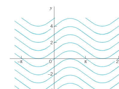
The ODE can be solved directly by integration on both sides. Indeed, using calculus, we obtain where cis an arbitrary constant. This is a family of solutions. Each value of c, for instance, 2.75 or 0 or gives one of these curves. Figure 3 shows some of them, for
䊏
⫺1, 0, 1, 2, 3, 4.
c⫽ ⫺3, ⫺2, ⫺8,
y⫽兰cos xdx⫽sin x⫹c, yr⫽dy>dx⫽cos x
y
x 0
–4
2π π
–π
4
2
–2
Fig. 3. Solutions y⫽sin x⫹cof the ODE yr⫽cos x
0 0.5 1.0 1.5 2.5
2.0
0 2 4 6 8 10 12 14 t y
Fig. 4B. Solutions of
in Example 3 (exponential decay)
yr⫽ ⫺0.2y
0 10 20 30 40
0 2 4 6 8 10 12 14 t y
Fig. 4A. Solutions of
in Example 3 (exponential growth)
yr⫽0.2y
E X A M P L E 3 (A) Exponential Growth. (B) Exponential Decay From calculus we know that has the derivative
Hence yis a solution of (Fig. 4A). This ODE is of the form With positive-constant k it can model exponential growth, for instance, of colonies of bacteria or populations of animals. It also applies to humans for small populations in a large country (e.g., the United States in early times) and is then known as
Malthus’s law.1We shall say more about this topic in Sec. 1.5.
(B)Similarly, (with a minus on the right) has the solution (Fig. 4B) modeling
exponential decay, as, for instance, of a radioactive substance (see Example 5). 䊏
y⫽ceⴚ0.2t, yr⫽ ⫺0.2
yr⫽ky. yr⫽0.2y
yr⫽dy dt ⫽0.2e
0.2t⫽0.2y. y⫽ce0.2t
We see that each ODE in these examples has a solution that contains an arbitrary constantc. Such a solution containing an arbitrary constant cis called a general solution of the ODE.
(We shall see that cis sometimes not completely arbitrary but must be restricted to some interval to avoid complex expressions in the solution.)
We shall develop methods that will give general solutions uniquely(perhaps except for notation). Hence we shall say thegeneral solution of a given ODE (instead of ageneral solution).
Geometrically, the general solution of an ODE is a family of infinitely many solution
curves, one for each value of the constant c. If we choose a specific c(e.g., or 0 or ) we obtain what is called a particular solutionof the ODE. A particular solution
does not contain any arbitrary constants.
In most cases, general solutions exist, and every solution not containing an arbitrary constant is obtained as a particular solution by assigning a suitable value to c. Exceptions to these rules occur but are of minor interest in applications; see Prob. 16 in Problem Set 1.1.
Initial Value Problem
In most cases the unique solution of a given problem, hence a particular solution, is obtained from a general solution by an initial condition with given values and , that is used to determine a value of the arbitrary constant c. Geometrically this condition means that the solution curve should pass through the point in thexy-plane. An ODE, together with an initial condition, is called an initial value problem. Thus, if the ODE is explicit, the initial value problem is of the form
(5)
E X A M P L E 4 Initial Value Problem Solve the initial value problem
Solution. The general solution is ; see Example 3. From this solution and the initial condition we obtain Hence the initial value problem has the solution . This is a particular solution.
More on Modeling
The general importance of modeling to the engineer and physicist was emphasized at the beginning of this section. We shall now consider a basic physical problem that will show the details of the typical steps of modeling. Step 1: the transition from the physical situation (the physical system) to its mathematical formulation (its mathematical model); Step 2: the solution by a mathematical method; and Step 3: the physical interpretation of the result. This may be the easiest way to obtain a first idea of the nature and purpose of differential equations and their applications. Realize at the outset that your computer (your CAS) may perhaps give you a hand in Step 2, but Steps 1 and 3 are basically your work. 䊏
y(x)⫽5.7e3x y(0)⫽ce0
⫽c⫽5.7.
y(x)⫽ce3x
y(0)⫽5.7. yr⫽dy
dx⫽3y,
y(x0)⫽y0. y
r
⫽f(x, y),y
r
⫽f(x, y),(x0, y0) y0
x0
y(x0)⫽y0, ⫺2.01
And Step 2 requires a solid knowledge and good understanding of solution methods available to you—you have to choose the method for your work by hand or by the computer. Keep this in mind, and always check computer results for errors (which may arise, for instance, from false inputs).
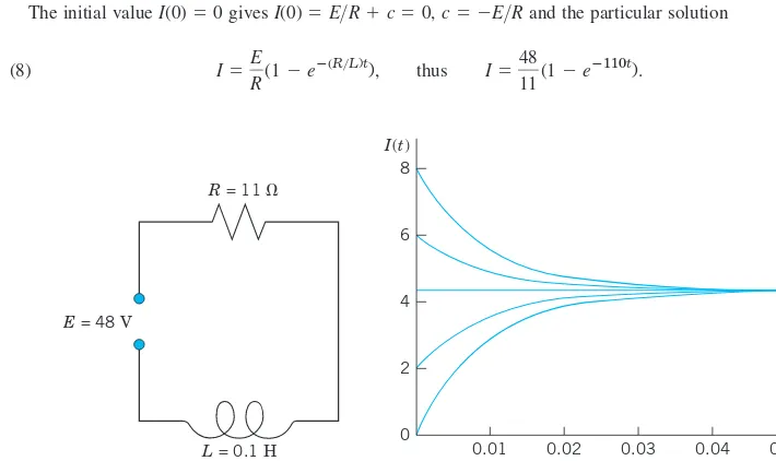
E X A M P L E 5 Radioactivity. Exponential Decay
Given an amount of a radioactive substance, say, 0.5 g (gram), find the amount present at any later time. Physical Information.Experiments show that at each instant a radioactive substance decomposes—and is thus decaying in time—proportional to the amount of substance present.
Step 1. Setting up a mathematical model of the physical process.Denote by the amount of substance still present at any time t. By the physical law, the time rate of change is proportional to . This gives the first-order ODE
(6)
where the constant k is positive, so that, because of the minus, we do get decay (as in [B] of Example 3). The value of k is known from experiments for various radioactive substances (e.g.,
approximately, for radium ).
Now the given initial amount is 0.5 g, and we can call the corresponding instant Then we have the initial condition This is the instant at which our observation of the process begins. It motivates the term initial condition(which, however, is also used when the independent variable is not time or when we choose a t other than ). Hence the mathematical model of the physical process is the initial value problem
(7)
Step 2. Mathematical solution.As in (B) of Example 3 we conclude that the ODE (6) models exponential decay and has the general solution (with arbitrary constant cbut definite given k)
(8)
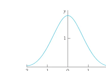
We now determine c by using the initial condition. Since from (8), this gives Hence the particular solution governing our process is (cf. Fig. 5)
(9)
Always check your result—it may involve human or computer errors! Verify by differentiation (chain rule!) that your solution (9) satisfies (7) as well as
Step 3. Interpretation of result.Formula (9) gives the amount of radioactive substance at time t. It starts from the correct initial amount and decreases with time because kis positive. The limit of yas is t:⬁ zero. 䊏
dy
dt⫽ ⫺0.5keⴚ kt⫽ ⫺k
ⴢ0.5eⴚkt⫽ ⫺ky, y(0)⫽0.5e0⫽0.5. y(0)⫽0.5:
(k⬎ 0). y(t)⫽0.5eⴚkt
y(0)⫽c⫽0.5. y(0)⫽c
y(t)⫽ceⴚkt. dy
dt ⫽ ⫺ky, y(0)⫽0.5. t⫽0
y(0)⫽0.5.
t⫽0. 226
88Ra
k⫽1.4ⴢ10ⴚ11 secⴚ1, dy
dt ⫽ ⫺ky
y(t) yr(t)⫽dy>dt
y(t)
0.1 0.2 0.3 0.4 0.5
0 y
0 0.5 1 1.5 2 2.5 3 t
Fig. 5. Radioactivity (Exponential decay, with k⫽1.5as an example)
1–8 CALCULUS
Solve the ODE by integration or by remembering a differentiation formula.
9–15 VERIFICATION. INITIAL VALUE PROBLEM (IVP)
(a) Verify that yis a solution of the ODE. (b) Determine from ythe particular solution of the IVP. (c) Graph the solution of the IVP.
9.
15. Find two constant solutions of the ODE in Prob. 13 by inspection.
16. Singular solution. An ODE may sometimes have an additional solution that cannot be obtained from the general solution and is then called a singular solution. The ODE is of this kind. Show by differentiation and substitution that it has the general solution and the singular solution
. Explain Fig. 6.
These problems will give you a first impression of modeling. Many more problems on modeling follow throughout this chapter.
17. Half-life. The half-life measures exponential decay. It is the time in which half of the given amount of radioactive substance will disappear. What is the half-life of (in years) in Example 5?
18. Half-life. Radium has a half-life of about 3.6 days.
(a) Given 1 gram, how much will still be present after 1 day?
(b) After 1 year?
19. Free fall. In dropping a stone or an iron ball, air resistance is practically negligible. Experiments show that the acceleration of the motion is constant
(equal to called the
acceleration of gravity). Model this as an ODE for , the distance fallen as a function of time t.If the motion starts at time from rest (i.e., with velocity ), show that you obtain the familiar law of free fall
20. Exponential decay. Subsonic flight. The efficiency of the engines of subsonic airplanes depends on air pressure and is usually maximum near ft. Find the air pressure at this height. Physical information. The rate of change is proportional to the pressure. At ft it is half its value at sea level. Hint.Remember from calculus
that if then Can you see
without calculation that the answer should be close to ?y0>4
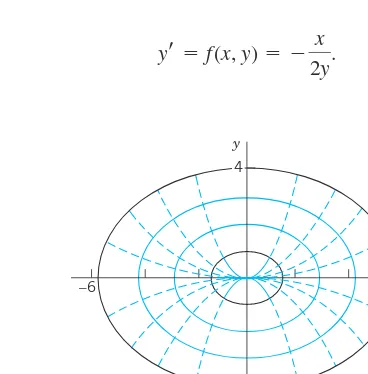
1.2
Geometric Meaning of
Direction Fields, Euler’s Method
A first-order ODE(1)
has a simple geometric interpretation. From calculus you know that the derivative of is the slope of . Hence a solution curve of (1) that passes through a point must have, at that point, the slope equal to the value of fat that point; that is,
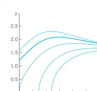
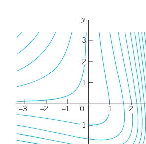
Using this fact, we can develop graphic or numeric methods for obtaining approximate solutions of ODEs (1). This will lead to a better conceptual understanding of an ODE (1). Moreover, such methods are of practical importance since many ODEs have complicated solution formulas or no solution formulas at all, whereby numeric methods are needed. Graphic Method of Direction Fields. Practical Example Illustrated in Fig. 7. We can show directions of solution curves of a given ODE (1) by drawing short straight-line segments (lineal elements) in the xy-plane. This gives a direction field (or slope field) into which you can then fit (approximate) solution curves. This may reveal typical properties of the whole family of solutions.
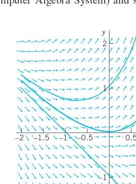
Figure 7 shows a direction field for the ODE (2)
obtained by a CAS (Computer Algebra System) and some approximate solution curves fitted in.
y
r
⫽y⫹xy
r
(x0)⫽f(x0, y0). yr
(x0)(x0, y0) y(x)
y(x)
y
r
(x) yr
⫽f(x, y)y
r
⫽
f
(
x
,
y
).
1 2
0.5 1 –0.5
–1 –1.5 –2
–1
–2 y
x
Fig. 7. Direction field of with three approximate solution curves passing through (0, 1), (0, 0), (0, ⫺1), respectively
If you have no CAS, first draw a few level curves const of , then parallel lineal elements along each such curve (which is also called an isocline, meaning a curve of equal inclination), and finally draw approximation curves fit to the lineal elements.
We shall now illustrate how numeric methods work by applying the simplest numeric method, that is Euler’s method, to an initial value problem involving ODE (2). First we give a brief description of Euler’s method.
Numeric Method by Euler
Given an ODE (1) and an initial value Euler’s method yields approximate
solution values at equidistant x-values namely,
(Fig. 8) , etc. In general,
where the step hequals, e.g., 0.1 or 0.2 (as in Table 1.1) or a smaller value for greater accuracy.
yn⫽yn⫺1⫹hf(xn⫺1, yn⫺1) y2⫽y1⫹hf(x1, y1)
y1⫽y0⫹hf(x0, y0)
x0, x1⫽x0⫹h, x2⫽x0⫹2h,Á, y(x0)⫽y0,
f(x, y) f(x, y)⫽
y
x
x0 x1
y0 y1 y(x1)
Solution curve
Error of y1
hf(x0,y0)
h
Fig. 8. First Euler step, showing a solution curve, its tangent at ( ), step hand increment hf(x0, y0)in the formula for y1
x0, y0
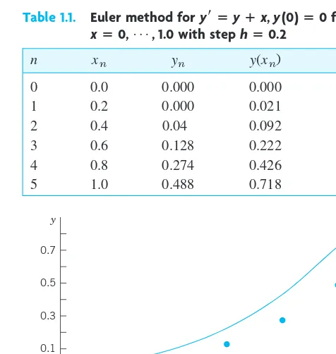
Table 1.1 shows the computation of steps with step for the ODE (2) and initial condition corresponding to the middle curve in the direction field. We shall solve the ODE exactly in Sec. 1.5. For the time being, verify that the initial value problem has the solution . The solution curve and the values in Table 1.1 are shown in Fig. 9. These values are rather inaccurate. The errors are shown in Table 1.1 as well as in Fig. 9. Decreasing hwould improve the values, but would soon require an impractical amount of computation. Much better methods of a similar nature will be discussed in Sec. 21.1.
y(xn)⫺yn y⫽ex⫺x⫺1
y(0)⫽0,
Table 1.1. Euler method for for with step hⴝ0.2
xⴝ0, Á, 1.0
y
r
ⴝyⴙx, y(0)ⴝ00.7
0.5
0.3
0.1
0 0.2 0.4 0.6 0.8 1 x
y
Fig. 9. Euler method: Approximate values in Table 1.1 and solution curve
n Error
0 0.0 0.000 0.000 0.000 1 0.2 0.000 0.021 0.021 2 0.4 0.04 0.092 0.052 3 0.6 0.128 0.222 0.094 4 0.8 0.274 0.426 0.152 5 1.0 0.488 0.718 0.230
y(xn)
yn
xn
1–8 DIRECTION FIELDS, SOLUTION CURVES Graph a direction field (by a CAS or by hand). In the field graph several solution curves by hand, particularly those passing through the given points .
1. 2. 3. 4. 5. 6. 7. 8.
9–10 ACCURACY OF DIRECTION FIELDS Direction fields are very useful because they can give you an impression of all solutions without solving the ODE, which may be difficult or even impossible. To get a feel for the accuracy of the method, graph a field, sketch solution curves in it, and compare them with the exact solutions.
9.
10. (Sol. )
11. Autonomous ODE. This means an ODE not showing x(the independent variable) explicitly. (The ODEs in Probs. 6 and 10 are autonomous.) What will the level curves f(x, y)⫽const (also called isoclines⫽curves
1y⫹52x⫽c yr⫽ ⫺5y1>2
yr⫽cos px
yr⫽ ⫺2xy, (0, 12), (0, 1), (0, 2) yr⫽ey>x, (2, 2), (3, 3) yr⫽sin2y, (0, ⫺0.4), (0, 1) yr⫽x⫺1>y, (1, 12)
yr⫽2y⫺y2, (0, 0), (0, 1), (0, 2), (0, 3) yr⫽1⫺y2, (0, 0), (2, 12)
yyr⫹4x⫽0, (1, 1), (0, 2) yr⫽1⫹y2, (14p, 1)
(x, y)
of equal inclination) of an autonomous ODE look like? Give reason.
12–15 MOTIONS
Model the motion of a body B on a straight line with velocity as given, being the distance of B from a point at time t.Graph a direction field of the model (the ODE). In the field sketch the solution curve satisfying the given initial condition.
12. Product of velocity times distance constant, equal to 2,
13.
14. Square of the distance plus square of the velocity equal to 1, initial distance
15. Parachutist. Two forces act on a parachutist, the attraction by the earth mg (m mass of person plus equipment, the acceleration of gravity) and the air resistance, assumed to be proportional to the square of the velocity v(t). Using Newton’s second law of motion (mass acceleration resultant of the forces), set up a model (an ODE for v(t)). Graph a direction field (choosing mand the constant of proportionality equal to 1). Assume that the parachute opens when v
Graph the corresponding solution in the field. What is the limiting velocity? Would the parachute still be sufficient if the air resistance were only proportional to v(t)?
⫽10 m>sec. ⫽
⫻
g⫽9.8 m>sec2 ⫽
1>12
Distance⫽Velocity⫻Time, y(1)⫽1 y(0)⫽2.
y⫽0
1.3
Separable ODEs. Modeling
Many practically useful ODEs can be reduced to the form
(1)
by purely algebraic manipulations. Then we can integrate on both sides with respect to x, obtaining
(2)
On the left we can switch to yas the variable of integration. By calculus, , so that
(3)
If fand gare continuous functions, the integrals in (3) exist, and by evaluating them we obtain a general solution of (1). This method of solving ODEs is called the method of separating variables, and (1) is called a separable equation, because in (3) the variables are now separated: xappears only on the right and yonly on the left.
E X A M P L E 1 Separable ODE
The ODE is separable because it can be written
By integration, or .
It is very important to introduce the constant of integration immediately when the integration is performed. If we wrote then and thenintroduced c, we would have obtained which
is not a solution (when c⫽0). Verify this. 䊏
y⫽tan x⫹c, y⫽tan x,
arctan y⫽x,
y⫽tan (x⫹c) arctan y⫽x⫹c
dy 1⫹y2⫽dx.
yr⫽1⫹y2
冮
g(y) dy⫽冮
f(x) dx⫹c.y
r
dx⫽dy冮
g(y) yr
dx⫽冮
f(x) dx⫹c.g(y) y
r
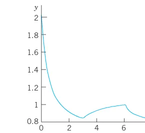
⫽f(x)16. CAS PROJECT. Direction Fields. Discuss direction fields as follows.
(a) Graph portions of the direction field of the ODE (2) (see Fig. 7), for instance,
Explain what you have gained by this enlargement of the portion of the field.
(b) Using implicit differentiation, find an ODE with the general solution Graph its direction field. Does the field give the impression that the solution curves may be semi-ellipses? Can you do similar work for circles? Hyperbolas? Parabolas? Other curves?
(c) Make a conjecture about the solutions of from the direction field.
(d) Graph the direction field of and some solutions of your choice. How do they behave? Why do they decrease for y ⬎ 0?
yr⫽ ⫺12y
yr⫽ ⫺x>y x2⫹9y2⫽c (y ⬎ 0).
⫺5⬉x⬉2, ⫺1⬉y⬉5.
17–20 EULER’S METHOD
This is the simplest method to explain numerically solving an ODE, more precisely, an initial value problem (IVP). (More accurate methods based on the same principle are explained in Sec. 21.1.) Using the method, to get a feel for numerics as well as for the nature of IVPs, solve the IVP numerically with a PC or a calculator, 10 steps. Graph the computed values and the solution curve on the same coordinate axes.
17.
18. 19.
Sol. 20.
Sol. y⫽1>(1⫹x)5
yr⫽ ⫺5x4y2, y(0)⫽1, h⫽0.2 y⫽x⫺tanh x