Department of Informatics Engineering Faculty of Industrial Technology

Department of Informatics Engineering

Faculty of Industrial Technology

Universitas Gunadarma

2018

References:

R. K. Nagle, E. B. Saff, A. D. Snider. (2012). Fundamentals of Differential Equations and Boundary Value Problems 6th Edition. New York: Addison-Wesley

349

Fourier Series

Mathematicians of the eighteenth century, including Daniel Bernoulli and Leonhard Euler, expressed the problem of the vibratory motion of a stretched string through partial differential equations that had no solu-tions in terms of “elementary funcsolu-tions.” Their resolution of this difficulty was to introduce infinite series of sine and cosine functions that satisfied the equations. In the early nineteenth century, Joseph Fourier, while studying the problem of heat flow, developed a cohesive theory of such series. Consequently, they were named after him. Fourier series and Fourier integrals are investigated in this chapter and Chapter 14. As you explore the ideas, notice the similarities and differences with the chapters on infinite series and improper integrals.

Periodic Functions

A function f(x) is said to have a period T or to be periodic with period T if for all x,f(x + T) = f(x), where T is a positive constant. The least value of T > 0 is called the least period or simply the period of f(x).

EXAMPLE 1. The function sin x has periods 2π, 4π, 6π, . . . , since sin(x + 2π), sin( + 4π), sin(x + 6π), . . . all equal sin x. However, 2π is the least period or the period of sin x.

EXAMPLE 2. The period of sin nx or cos nx, where n is a positive integer, is 2π/n.

EXAMPLE 3. The period of tan x is π.

EXAMPLE 4. A constant has any positive number as period.

Other examples of periodic functions are shown in the graphs of Figure 13.1(a), (b), and (c).

Figure 13.1

Fourier Series

Letf(x) be defined in the interval (–L, L) and outside of this interval by f(x + 2L) = f(x); i.e., f(x) is 2L -periodic. It is through this avenue that a new function on an infinite set of real numbers is created from the image on (–L, L). The Fourier series or Fourier expansion corresponding to f(x) is given by

f(x)

(a)

x

0

To correlate the coefficients with the expansion, see the following Examples 1 and 2.

Orthogonality Conditions for the Sine and Cosine Functions

Notice that the Fourier coefficients are integrals. These are obtained by starting with the series (1) and em-ploying the following properties called orthogonality conditions:

(a) Lcos cos 0 if and if

An explanation for calling these orthogonality conditions is given on Page 355. Their application in de-termining the Fourier coefficients is illustrated in the following pair of examples and then demonstrated in detail in Problem 13.4.

EXAMPLE 1. To determine the Fourier coefficient a₀, integrate both sides of the Fourier series (1) and em-ploy the orthogonality conditions (2).

}

and then integrate. Using the

or-thogonality conditions (3)a and (3)c, we obtain 1

Then the series (1) with Fourier coefficients converges to (a) f(x) if x is a point of continuity

(b) ( 0) ( 0)

2

f x+ + f x−

if x is a point of discontinuity

Heref(x + 0) and f(x – 0) are the right- and left-hand limits of f(x) at x and represent

0 lim

ε → + f(x + ⑀) and ε → +lim0

f(x – ⑀_{), respectively. For a proof, see Problems 13.18 through 13.23.}

The conditions 1, 2, and 3 imposed on f(x) are sufficient but not necessary, and are generally satisfied in practice. There are at present no known necessary and sufficient conditions for convergence of Fourier series. It is of interest that continuity of f(x) does not alone ensure convergence of a Fourier series.

Odd and Even Functions

A function f(x) is called odd if f(–x) = –f(x). Thus, x3_,x5 _{– 3x}3 _{+ 2x, sin x, and tan 3x are odd functions.}

A function f(x) is called even if f(–x) = f(x). Thus, x4_{, 2x}6 _{– 4x}2 _{+ 5, cos x, and e}x _{+ e}–x _{are even} func-tions.

The functions portrayed graphically in Figure 13.1(a) and (b) are odd and even, respectively, but that of Figure 13.1(c) is neither odd nor even.

In the Fourier series corresponding to an odd function, only sine terms can be present. In the Fourier series corresponding to an even function, only cosine terms (and possibly a constant, which we shall consider a cosine term) can be present.

Half Range Fourier Sine or Cosine Series

A half range Fourier sine or cosine series is a series in which only sine terms or only cosine terms are present, respectively. When a half range series corresponding to a given function is desired, the function is generally defined in the interval (0, L) [which is half of the interval (–L, L), thus accounting for the name half range] and then the function is specified as odd or even, so that it is clearly defined in the other half of the interval, namely, (–L, 0). In such case, we have

0 2

0, ( ) sin for

2

0, ( ) cos for

L

n n _L

L

n n

n x

a b f x dx half range sine series

L L

n x

b a f x dx half range consine series

L L

π

π −

 = =

 

 = =



∫

∫

(4)

Parseval’s Identity

Ifan and bn are the Fourier coefficients corresponding to f(x) and if f(x) satisfies the Dirichlet conditions, then

2

2

2 0 2

1 1

{ ( )} ( )

2 L

n n

L

n

a

f x dx a b

L

∞

− = +

∑

₌ +

∫

(5)

(See Problem 13.13.)

Differentiation and Integration of Fourier Series

Theorem The Fourier series corresponding to f(x) may be integrated term by term from a to and the result-ing series will converge uniformly to x ( )

a f x dx

∫

provided that F(x) is piecewise continueus in –L < x < L and both a and x are in this interval.

Complex Notation for Fourier Series

Using Euler’s identities,

eiθ _{= cos θ + i sinθ,e}–iθ _{= cos θ – i sin θ (6)}

wherei = −1 (see Problem 11.48), the Fourier series for f(x) can be written as

/

( ) in x L

n n

f x c e π

∞

=−∞

=

∑

(7)

where

/ 1

( ) 2

L

in x L n

L

c f x e dx

L

π − −

=

_∫

(8)

In writing the equality (7), we are supposing that the Dirichlet conditions are satisfied and, further, that f(x) is continuous at x. If f(x) is discontinuous at x, the left side of (7) should be replaced by

( ( 0) ( 0)

. 2

f x+ + f x−

Boundary-Value Problems

Boundary value problems seek to determine solutions of partial differential equations satisfying certain prescribed conditions called boundary conditions. Some of these problems can be solved by use of Fourier series (see Problem 13.24).

EXAMPLE. The classical problem of a vibrating string may be idealized in the following way. See Figure 13.2.

Suppose a string is tautly stretched between points (0, 0) and (L, 0). Suppose the tension F is the same at every point of the string. The string is made to vibrate in the xy plane by pulling it to the parabolic position g(x) = m(Lx – x2_{) and releasing it (m is a numerically small positive constant). Its equation will be of the form}

y = f(x, t). The problem of establishing this equation is idealized by (a) assuming that the constant tension F is so large as compared to the weight wL of the string that the gravitational force can be neglected, (b) the displacement at any point of the string is so small that the length of the string may be taken as L for any of its positions, and (c) the vibrations are purely transverse.

The force acting on a segment PQ is

2 2 ,

w y

x

g t

∂ ∆

∂ x < x1 < x + ∆x, g≈ 32 ft per sec2

If α and β are the angles that F makes with the horizontal, then the vertical difference in tensions is F(sinα – sin β). This is the force producing the acceleration that accounts for the vibratory motion.

Figure 13.2

Now

F{sinα – sin β} = F

2 2

tan tan

1 tan 1 tan

α β

α β

 

 ₋ 

 

+ +

 

 

≈F{tanα – tan β} F y(x x t, ) y( , )x t

x x

∂ ∂

 

= _ + ∆ − _

∂ ∂

 

where the squared terms in the denominator are neglected because the vibrations are small. Next, equate the two forms of the force, i.e.,

2 2

( , ) ( , )

y y w y

F x x t x t x

x x g t

∂ ∂ ∂

 _{+ ∆ −} _{= ∆}

_{∂ ∂}  _∂

 

divide by ∆x, and then let ∆x→ 0. After letting Fg,

w

α = the resulting equation is

2 2

2

2 2

y y

t α x

∂ ₌ ∂

∂ ∂

This homogeneous second partial derivative equation is the classical equation for the vibrating string. Associated boundary conditions are

y(0,t) = 0, y(L, t) = 0, t > 0 The initial conditions are

2

( , 0) ( ), y( , 0) 0, 0

y x m Lx x x x L

t ∂

= − = < <

∂

The method of solution is to separate variables, i.e., assume y(x, t) = G(x)H(t) Then, upon substituting,

G(x)H″ (t) = α2_{G″ (x)H(t)} Separating variables yields

" " 2

, ,

G H

k k

G = H =α where k is an arbitrary constant Since the solution must be periodic, trial solutions are

1 2

3 4

( ) sin cos , 0

( ) sin cos

G x c k x c k x

H t c α k t c α k t

= − + − <

= − + −

Therefore,

1 2 3 4

[ sin cos ][ sin cos ]

y=GH= c −k x+c −k x c α −k t+c α −k t

The initial condition y = 0 at x = 0 for all t leads to the evaluation c2 = 0.

Thus,

c1⫽ 0, as that would imply y = 0 and a trivial solution. The next-simplest solution results from the

choice k n , sincey c₁sinn x c₃sin n t c₄cos n t

∂ can be considered.

1sin 3 cos 4 sin

The remaining initial condition is

y(x, 0) = m(Lx – x2_{), 0 < x < L} When it is imposed,

2

However, this relation cannot be satisfied for all x on the interval (0, L). Thus, the preceding extensive analysis of the problem of the vibrating string has led us to an inadequate form:

1 4 sin cos

and an initial condition that is not satisfied. At this point the power of Fourier series is employed. In particu-lar, a theorem of differential equations states that any finite sum of a particular solution also is a solution. Generalize this to infinite sum and consider

1

with the initial condition expressed through a half range sine series, i.e.,

2

According to the formula on Page 351 for the coefficient of a half range sine series,

2

Application of integration by parts to the second integral yields

When integration by parts is applied to the two integrals of this expression and a little algebra is employed, the result is

2 3 4

(1 cos )

( )

n

L

b n

nπ π

= −

Therefore,

1

sin cos

n n

n n

y b x t

L L

π π

α ∞

= =

∑

with the coefficients b_n defined previously.

Orthogonal Functions

Two vectors A and B are called orthogonal (perpendicular) if A · B = 0 or or A₁B₁ + A₂B₂ + A₃B₃ = 0, where

A = A₁i + A₂j + A₃k and B = B₁i + B₂j + B₃k. Although not geometrically or physically evident, these ideas can be generalized to include vectors with more than three components. In particular, we can think of a function—say, A(x)—as being a vector with an infinity of components (i.e., an infinite dimensional vector), the value of each component being specified by substituting a particular value of x in some interval (a, b). It is natural in such case to define two functions, A(x) and B(x), as orthogonal in (a, b) if

( ) ( ) 0

b

a A x B x dx=

∫

(9)

A vector A is called a unit vector or normalized vector if its magnitude is unity, i.e., if A · A = A2 _{= 1.}

Extending the concept, we say that the function A(x) is normal or normalized in (a, b) if

2

{ ( )} 1

b

a A x dx=

∫

(10)

From this, it is clear that we can consider a set of functions {φk (x)},k = 1, 2, 3, . . . , having the properties

( ) b

m

aφ x

∫

) ( )φ_n x dx=0 m≠n (11)

2

{ ( )} 1 1, 2, 3,...

b m

a φ x dx= m=

∫

(12)

In such case, each member of the set is orthogonal to every other member of the set and is also normalized. We call such a set of functions an orthonormal set.

Equations (11) and (12) can be summarized by writing

( ) b

m

aφ xφ

∫

φ_n( )x dx=δ_mn (13)

whereδmn, called Kronecker’s symbol, is defined as 0 if m⫽n and 1 if m = n.

Just as any vector r in three dimensions can be expanded in a set of mutually orthogonal unit vectors i, j,

k in the form r = c1i + c2j + c3k, so we consider the possibility of expanding a function f(x) in a set of

ortho-normal functions, i.e.,

1

( ) n n( )

n

f x cφ x a x b

∞

=

=

∑

≤ ≤ (14)

SOLVED PROBLEMS

Fourier Series

13.1. Graph each of the following functions.

(a) ( ) 3 0 5 Period 10

3 5 0

x f x

x < < 

=_{− − < <} =



Figure 13.3

Since the period is 10, that portion of the graph in –5 < x < 5 (indicated by heavy lines in Figure 13.3) is extended periodically outside this range (indicated by dashed lines). Note that f(x) is not defined at x = 0, 5, –5, 10, –10, 15, –15, and so on. These values are the discontinuities of f(x).

(b) ( ) sin 0 Period = 2

0 2

x x

f x

x π

π

π π

< < 

= 

< < 

Figure 13.4

Refer to Figure 13.4. Note that f(x) is defined for all x and is continuous everywhere.

(c)

0 0 2

( ) 1 2 4 Period 6

0 4 6

x

f x x

x ≤ < 



= ≤ < =

 _{≤ <} 

Fig.13.5

Refer to Figure 13.5. Note that f(x) is defined for all x and is discontinuous at x = ±2, ±4, ±8, ±10, ±14, . . . .

13.2. prove sink x cosk x 0 1, 2, 3,...

L L

L L

-L dx -L dx if k

π ₌ π _{= =}

k x k x

sin cos sin sin

1

( ) cos cos

cos cos cos sin

if 0

and integrating from –L to L, using Problem 13.3, we have

( ) sin sin

sin cos cos sin

L L

Note that in (a), (b), and (c), interchange of summation and integration is valid because the series is as-sumed to converge uniformly to f(x) in (–L,L). Even when this assumption is not warranted, the coefficients a_m and b_m as obtained are called Fourier coefficients corresponding to f(x), and the corresponding series with these values of a_m and b_m is called the Fourier series corresponding to f(x). An important problem in this case is to investigate conditions under which this series actually converges to f(x). Sufficient conditions for this convergence are the Dirichlet conditions established in Problems 13.18 through 13.23.

13.5. (a) Find the Fourier coefficients corresponding to the function

0 5 0

(b) Write the corresponding Fourier series.

(c) How should f(x) be defined at x = –5, x = 0, and x = 5 in order that the Fourier series will converge to f(x) for –5 < x < 5?

Figure 13.6

(b) The corresponding Fourier series is

Period = 2L = 2π and L = π. Choosing c = 0, we have

(b) If the period is not specified, the Fourier series cannot be determined uniquely in general.

13.7. Using the results of Problem 13.6, prove that 1₂ 1₂ 1₂

By the Dirichlet conditions, the series converges at x = 0 to 1

2 (0 + 4π

Odd and even functions, half range Fourier series

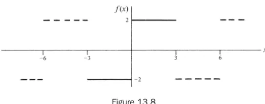
13.8. Classify each of the following functions according to whether they are even, odd, or neither even nor odd.

Figure 13.8

From Figure 13.9, it is seen that the function is neither even nor odd.

Figure 13.9

(c) f(x) = x(10 –x), 0 < x < 10 Period = 10

From Figure 13.10 below the function is seen to be even.

Figure 13.10

13.9. Show that an even function can have no sine terms in its Fourier expansion.

Method 1: No sine terms appear if b_n = 0, n = 1, 2, 3, . . . . To show this, let us this, let us write

0

0

1 1 1

( ) sin ( ) sin ( ) sin

L L

n _{L L}

n x n x n x

b f x dx f x dx f x dx

L L L L L L

π π π

− −

=

_∫

=

_∫

+

_∫

(1)

If we make the transformation x = –u in the first integral on the right of Equation (1), we obtain

0

0 0

0 0

1 1 1

( ) sin ( ) sin ( ) sin

1 1

( ) sin ( ) sin

L L

L

L L

n x n u n u

f x dx f u du f u du

L L L L L L

n u n u

f u du f x dx

L L L L

π π π

π π

−

 

= − _− _ = − −

= − = −

∫

∫

∫

∫

∫

(2)

where we have used the fact that for an even function f(–u) = f(u) and in the last last step that the dummy variable of integration u can be replaced by any other symbol, in particular, x. Thus, from Equation (1), using Equation (2), we have

0 0

1 1

( ) sin ( ) sin 0

L L

n

n x n u

b f x dx f x dx

L L L L

π π

Method 2: Assume

cos sin cos sin

2 n n n 2 n n n

and no sine terms appear.

In a similar manner, we can show that an odd function has no cosine terms (or constant term) in its Fourier expansion.

(b) This follows by Method 1 of Problem 13.9.

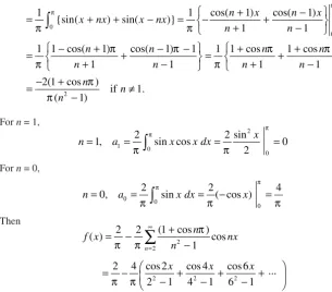
13.11. Expand f(x) = sin x, 0 < x < π, in a Fourier cosine series.

0

Figure 13.13

where the integral is assumed to exist.

If 0 from –L to L (which is justified since the series is uniformly convergent), we obtain

{

where we have used the results

:

obtained from the Fourier coefficients.

The required result follows on dividing both sides of Equation (1) by L. Parseval’s identity is valid under less restrictive conditions than that imposed here.

13.14. (a) Write Parseval’s identity corresponding to the Fourier series of Problem 13.12(b). (b) Determine from (a)

Then Parseval’s identity becomes

2

13.15. Prove that for all positive integers M,

2

since the integrand is nonnegative. Expanding the integrand, we obtain

2 2

Also, squaring Equation (1) and integrating from –L to L, using Problem 13.3, we find

2

Substitution of Equations (4) and (5) into Equation (3) and dividing by L yields the required result. Taking the limit as M→⬁_{, we obtain Bessel’s inequality}

2

If the equality holds, we have Parseval’s identity (Problem 13.13). ... ...

... ...

... ... ...

We can think of SM(x) as representing an approximation to f(x), while the left-hand side of Equation (2), divided by 2L, represents the mean square error of the approximation. Parseval’s identity indicates that as M→⬁_{, the mean square error approaches zero, while Bessels’ inequality indicates the possibility that this}

mean square error does not approach zero.

The results are connected with the idea of completeness of an orthonormal set. If, for example, we were to leave out one or more terms in a Fourier series (cos 4πx/L, for example), we could never get the mean square error to approach zero no matter how many terms we took. For an analogy with three-dimensional vectors, see Problem 13.60.

Differentiation and integration of Fourier series

13.16. (a) Find a Fourier series for f(x) = x2_{, 0 < x < 2, by integrating the series of Problem 13.12(a). (b) Use (a) to}

(a) From Problem 13.12(a).

4 1 2 1 3

Integrating both sides from 0 to x (applying the theorem of Page 352) and multiplying by 2, we find

2

(b) To determine C in another way, note that Equation (2) represents the Fourier cosine series for x2 _{in 0 < x} < 2. Then, since L = 2 in this case,

13.17. Show that term-by-term differentiation of the series in Problem 13.12(a) is not valid.

Term-by-term differentiation yields 2 cos cos2 cos3 .

2 2 2

series does not approach 0, the series does not converge for any value of x.

Convergence of Fourier series

(a) We have cos sin1 1 sin 1 sin 1 .

2, the required result follows.

(b) Integrating the result in (a) from –π to 0 and 0 to π, respectively, gives the required results, since the in-tegrals of all the cosine terms are zero.

13.19. Prove that lim ( ) sin lim ( ) cos 0 if ( )

This follows at once from Problem 13.15, since if the series

2

The result is sometimes called Riemann’s theorem.

13.20. Prove that lim ( ) sin 1 0 if ( )

∫

is piecewise continuous.

We have

2 x, respectively, which are piecewise continuous if f(x) is.

The result can also be proved when the integration limits are a and b instead of –π and π.

Using the formulas for the Fourier coefficients with L = π, we have

Then 2π, in particular, –π,π. Thus, we obtain the required result.

13.22. Prove that

(

( 0) ( 0)

)

₁ 0

(

( ) ( 0)

)

₁

Subtracting Equation (2) from Equation (1) yields the required result.

Also,

since, by hypothesis, f′(x) is piecewise continuous so that the right-hand derivative of f(x) at each x exists.

Thus, ( ) ( 0)

Then, from Problems 13.20 and 13.22, we have

( 0) ( 0) ( 0) ( 0)

A method commonly employed in practice is to assume the existence of a solution of the partial differen-tial equation having the particular form U(x,t) = X(x)T(t), where X(x) and T(t) are functions of x and t, respec-tively, which we shall try to determine. For this reason, the method is often called the method of separation of variables.

Substitution in the differential equation yields

2 Equation (2) can be written as

2

In Problem 13.47 we see that if c > 0, a solution satisfying the given boundary conditions cannot exist. Let us thus assume that c is a negative constant, which we write as –λ2_{. Then, from Equation (3), we} obtain two ordinary differentiation equations

2

2

We now seek to determine A and B so that Equation (6) satisfies the given boundary conditions. To satisfy the condition U(0,t) = 0, we must have

2

( ) 0 or 0

s t

e−λ A = A= (7)

so that Equation (6) becomes

( , )

SinceB = 0 makes the solution (8) identically zero, we avoid this choice and instead take

sin 2 0, i.e., 2 or =

Substitution in Equation (8) now shows that a solution satisfying the first two boundary conditions is

2 2

where we have replaced B by Bm, indicating that different constants can be used for different values of m. If we now attempt to satisfy the last boundary condition U(x, 0) = x, 0 < x < 2, we find it to be impossible using Equation (11). However, upon recognizing the fact that sums of solutions having the form (11) are also solutions (called the principle of superposition), we are led to the possible solution

2 2 series. The solution to this is given in Problem 13.12(a), from which we see that B_m 4

mπ

which is a formal solution. To check that Equation (14) is actually a solution, we must show that it satisfies the partial differential equation and the boundary conditions. The proof consists in justification of term-by-term differentiation and use of limiting procedures for infinite series and may be accomplished by methods of Chapter 11.

The boundary value problem considered here has an interpretation in the theory of heat conduction. The

Orthogonal functions

13.25. (a) Show that the set of functions

2 2 3 3

(b) Determine the corresponding normalizing constants for the set in (a) so that the set is orthonormal in (–L,L).

(a) This follows at once from the results of Problems 13.2 and 13.3.

(b) By Problem 13.3,

Thus, the required orthonormal set is given by

1 1 1 1 2 1 2

Letx = π in the Fourier series obtained in Problem 13.26. Then

...

...

2 2 2 2 2 2

This result is of interest since it represents an expansion of the contangent into partial fractions.

By the Weierstrass M test, the series on the right of Equation (1) converges uniformly for 0 < α <x < 1

called the infinite product for sin x, which can be shown valid for all x. The result is of interest since it corre-sponds to a factorization of sin x in a manner analogous to factorization of a polynomial.

13.28. Prove that 2 2 4 4 6 6 8 8 .

Taking reciprocals of both sides, we obtain the required result, which is often called Wallis’s product.

SUPPLEMENTARY PROBLEMS

Fourier Series

13.29. Graph each of the following functions and find their corresponding Fourier series using properties of even and odd functions wherever applicable.

(a) ( ) 8 0 2 Period 4

13.30. In each part of Problem 13.29, tell where the discontinuities of f(x) are located and to what value the series converges at the discontunities.

Ans. (a) x = 0, ±2, ±4, . . . ; 0 (c) x = 0, ±10, ±20, . . . ; 20 Problem 13.32, explaining the similarities and differences, if any.

Ans. Answer is the same as in Problem 13.32.

13.34. Expand ( ) 0 4

13.36. Use the preceding problem to show that

13.37. Show that 1₃ 1₃ 1₃ 1₃ 1₃ 1₃

Differentiation and integration of Fourier series

13.38. (a) Show that for –π < x < π,

13.40. By differentiating the result of Problem 13.35(b), prove that for 0 < x < π,

2 2 2

13.41. By using Problem 13.35 and Parseval’s identity, show that

Boundary value problems where 0 < x < 4, t > 0. (b) Give a possible physical interpretation of the problem and solution.

Ans. (a) U(x, t) = 3e –2π2_{t sin πx – 2e} –50π2_{t sin 5πx}

interpret and interpret physically.

Ans. 2 2/ 36 satisfying the boundary value problem.

13.48. A flexible string of length π is tightly stretched between points x = 0 and x = = π on the xaxis, its ends are fixed at these points. When set into small transverse vibration, the displacement Y(x, t) from the the xaxis of

any point x at time t is given by

(a) Find a solution of this equation (sometimes called the wave equation) with a2 _{= 4 which satisfies the} conditionsY(0,t) = 0, Y(π,t) = 0, Y(x, 0) = 0.1 sin x + 0.01 sin 4x,Yt(x, 0) = 0 for 0 < x < π,t > 0. (b) Interpret physically the boundary conditions in (a) and the solution.

Ans. (a) Y(x, t) = 0.1 sin x cos 2t + 0.01 sin 4x cos 8t

13.49. (a) Solve the boundary value problem

2 2

13.50. Solve the boundary value problem

2

13.51. Give a physical interpretation to Problem 13.50.

13.52. Solve Problem 13.49 with the boundary conditions for Y(x, 0) and Yt(x, 0) interchanged; i.e., Y(x,) = 0,

Miscellaneous Problems

13.54. If –π < x < π and α⫽ _{0, ±1. ±2, . . . , prove that}

2 2 2 2 2 2

sin sin 2 sin 2 3sin 3

2 sin 1 2 3

x x x x

π α

απ = −α − −α + −α − . . .

13.55. If –π < x < π, prove that

(a) sinh sin_{2 2} 2 sin 2_{2 2} 3sin 3_{2 2}

2 sinh 1 2 3

x x x x

π α

απ =α + −α + +α + −. . .

(b) cosh 1 ₂cos₂ cos 2_{2 2}

2 sinh 2 1 2

x x x

π α α α

απ = α α− + +α + −. . .

13.56. Prove that

2 2 2

2 2 2

sinh 1 1 1

(2 ) (3 )

x x x

x x

π π π

   

= _ + _ + _ + _

 _  . . . .

13.57. Prove that

2 2 2

2 2 2

4 4 4

cos 1 1 1

(3 ) (5 )

x x x

x

π π π

     

=_ − _{ } − _{ } − _

 _{ }   . . . . [Hint: cos

x = (sin 2x)/(2 sin x).]

13.58. Show that

(a) 2 1 3 5 7 9 22 13 15

2 2 6 6 10 10 14 14 2

⋅ ⋅ ⋅ ⋅ ⋅ ⋅ ⋅ =

⋅ ⋅ ⋅ ⋅ ⋅ ⋅ ⋅ L

L . . .

. . .

(b) 2 4 4 4 8 8 12 12 16 16

3 5 7 9 11 13 15 17

π _{= } ⋅ ⋅ ⋅ ⋅ ⋅ ⋅ ⋅_{⋅ ⋅ ⋅ ⋅ ⋅ ⋅ ⋅} 

 

L L . . . . . .

13.59. Let r be any three-dimensional vector. Show that (a) (r · i)2 _{+ (r · j)}2 < _(r)2 _{and (b) (r · i)}2 _{+ (r · j)}2 _{+ (r · k)}2 =r2 _{and discuss these with reference to Parseval’s identity.}

13.60. If {φn (x)}, n = 1, 2, 3, . . . is orthonormal in (a, b, prove that

2

1

( ) ( )

b

n n a

n

f x cφ x

∞

=

 ₋ 

 



∑



∫

dx is a minimum

when n b ( )

a

377

Fourier Integrals

Fourier integrals are generalizations of Fourier series. The series representation a0

2 + ancos

nπx L +bnsin

nπx L ⎧

⎨ ⎩

⎫ ⎬ ⎭

n=1 ∞

∑

of a function is a periodic form on –⬁ < x < ⬁ obtained by generating the coefficients from the function’s definition on the least period [–L, L]. If a function defined on the set of all real numbers has no period, then an analogy to Fourier integrals can be envisioned as letting L→⬁ and replacing the integer valued index n by a real valued function α. The coefficients an and bn then take the form A(α) and B(α). This mode of thought leads to the following definition. (See Problem 14.8.)

The Fourier Integral

Let us assume the following conditions on f(x):

1. f(x) satisfies the Dirichlet conditions (Page 350) in every finite interval (–L, L).

2. f(x)

−∞ ∞

∫

dxconverges; i.e., f(x) is absolutely integrable in (–⬁,⬁).

ThenFourier’s integral theorem states that the Fourier integral of a function f is

f(x)= {A(α) cosαx

0 ∞

∫

+B(α) sinαx}dα (1)

where

A(α)= 1

π −∞f(x) cosαx dx ∞

∫

B(α)= 1

π −∞f(x) sinαx dx ∞

∫

⎧ ⎨ ⎪⎪ ⎩ ⎪ ⎪

⎫ ⎬ ⎪⎪ ⎭ ⎪ ⎪

(2)

A(α) and B(α) with –⬁ < α < ⬁ are generalizations of the Fourier coefficients a

n and bn. The right-hand side of Equation (1) is also called a Fourier integral expansion of f. (Since Fourier integrals are improper integrals, a review of Chapter 12 is a prerequisite to the study of this chapter.) The result (1) holds if x is a

point of continuity of f(x). If x is a point of discontinuity, we must replace f(x) by f(x+0)+ f(x−0)

2 , as in

the case of Fourier series. Note that these conditions are sufficient but not necessary.

In the generalization of Fourier coefficients to Fourier integrals, a0 may be neglected, since whenever

f(x)

−∞ ∞

∫

dxexists,

|a₀|= 1

L −Lf(x)dx L

Equivalent Forms of Fourier’s Integral Theorem

Fourier’s integral theorem can also be written in the forms

f(x)= 1

These results can be simplified somewhat if f(x) is either an odd or an even function, and we have

0 0

An entity of importance in evaluating integrals and solving differential and integral equations is introduced in the next paragraph. It is abstracted from the Fourier integral form of a function, as can be observed by putting Equation (4) in the form

f(x)= 1

and identifying the parenthetic expression, as F(α). The following Fourier transforms result.

Fourier Transforms

From Equation (4) it follows that

F(α)= 1

Note: The constants preceding the integral signs in Equations (7) and (8) were here taken as equal to

Iff(x) is an odd function, Equation (6) yields

When the product of Fourier transforms is considered, a new concept called convolution comes into being, and in conjunction with it, a new pair (function and its Fourier transform) arises. In particular, if F(α) and G(α) are the Fourier transforms of f and g, respectively, and the convolution of f and g is defined to be

It may be said that multiplication is exchanged with convolution. Also “the Fourier transform of the con-volution of two functions, f and g is the product of their Fourier transforms,” i.e.,

T(f_*g)=G(f)T(g)

[F(α)G(α) and f∗g) are demonstrated to be a Fourier transform pair in Problem 14.29.] Now equate the representations of f∗g expressed in Equations (11) and (13), i.e.,

1 Then Equation (15) takes the form

| f(u) |2 _du=

This is Parseval’s theorem for Fourier integrals.

SOLVED PROBLEMS

The Fourier integral and Fourier transforms

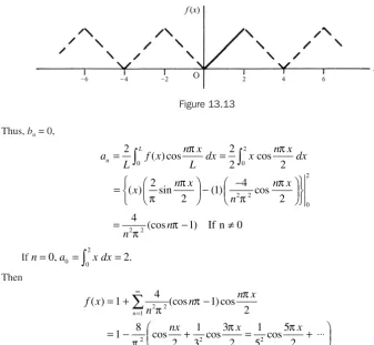
14.1. _{(a) Find the Fourier transform of f(x)}= 1 |x| < a

Figure 14.1 Figure 14.2

14.2. _{(a) Use the result of Problem 14.1 to evaluate} sinαa cosαx

(a) From Fourier’s integral theorem, if

F(α)= 1 Then, from Problem 14.1,

1

The left side of Equation (1) is equal to

1

The integrand in the second integral of Equation (2) is odd, and so the integral is zero. Then from Equa-tions (1) and (2), we have

(b) If x = 0 and a = 1 in the result of (a), we have since the integrand is even.

14.3. _If f(x) is an even function, show that (a) F(α)= 2 tion (1) is zero, and the result can be written

F(α)= 2 in (a), the required result follows.

A similar result holds for odd functions and can be obtained by replacing the cosine by the sine.

14.4. _{Solve the integral equation} f(x) cosαx dx= 1− α 0< α <1

14.5. _{Use Problem 14.4 to show that} sin 2_u

As obtained in Problem 14.4,

2

But this integral can be written as 2 sin 2 that the required result follows.

Then

14.7. _{Verify Parseval’s identity for Fourier integrals for the Fourier transforms of Problem 14.1.}

We must show that

{f(x)}2_dx=

This is equivalent to

(1)2dx= 2

Proof of the Fourier integral theorem

14.8. _{Present a heuristic demonstration of Fourier’s integral theorem by use of a limiting form of Fourier series.}

Let

Then, by substitution (see Problem 13.21),

f(x)= 1

∫

converges, the first term on the right of Equation (2) approaches zero as

L→⬁, while the remaining part appears to approach

This last step is not rigorous and makes the demonstration heuristic.

where we have written

F(α)= 1

π 0 f(u) cosα(u−x)du ∞

∫

(5)

But the limit (4) is equal to

f(x)= F(α)dα which is Fourier’s integral formula.

This demonstration serves only to provide a possible result. To be rigorous, we start with the integral

1/π ∫⬁ 0dα ∫

⬁

–⬁f(u) cos α(u – x)dx

and examine the convergence. This method is considered in Problems 14.9 through 14.12.

14.9. _{Prove that}

14.10. _{Riemann’s theorem states that if} F(x) is piecewise continuous in (a, b), then

lim

α→∞ aF(x) sinαx dx=0 b

∫

with a similar result for the cosine (see Problem 14.32). Use this to prove that

(a) lim (a) Using Problem 14.9(a), it is seen that a proof of the given result amounts to proving that

lim

υ is piecewise continuous

in (0, L), since 0

lim

n→ + F(υ) exists and f(x) is piecewise continuous.

14.11. _{If f(x) satisfies the additional condition that | f(x) |dx} −∞

∞

∫

converges, prove that (a) lim

L sufficiently large so that the required result follows.

This result follows by reasoning exactly analogous to that in (a).

14.12. _{Prove Fourier’s integral formula where} f(x) satisfies the conditions stated on Page 377.

We must prove that lim

L→∞

Miscellaneous problems

We proceed as in Problem 13.24. A solution satisfying the partial differential equation and the first bound-ary condition is given by Be–λ2_{t sin λx. Unlike Problem 13.24, the boundary conditions do not prescribe the} specific values for λ, so we must assume that all values of λ are possible. By analogy with that problem, we sum over all possible values of λ, which corresponds to an integration in this case, and are led to the possible solution

U(x, 1)= B(λ)

0 ∞

∫

e−λ2tsinλxdλ (1)

whereB(λ) is undetermined. By the second condition, we have

B(λ) sinλxdλ = 1 0<x<1

from which we have, by Fourier’s integral formula,

B(λ)= 2

so that, at least formally, the solution is given by

U(x, 1)= 2 Lettingx = 2u and using Problem 12.32, the integral becomes

2

which proves the required result.

14.15. _{Solve the integral equation}

y(x)=g(x)+ y(u)r(x−u)du respectively. Then, taking the Fourier transform of both sides of the given integral equation, we have, by the convolution theorem,

SUPPLEMENTARY PROBLEMS

The Fourier integral and Fourier transforms

14.16. _{(a) Find the Fourier transform of f(x)}= 1 / 2∈ |x|< ∈

0 |x|> ∈

⎧ ⎨

⎩ . (b) Determine the limit of this transform as

⑀→ 0+ and discuss the result.

⎩⎪ , find (a) the Fourier since transform and (b) the Fourier cosine transform of f(x).

In each case, obtain the graph of f(x) and its transform.

Ans.(a) 2 the result in (a). (c) Explain from the viewpoint of Fourier’s integral theorem why the result in (b) does not hold for m = 0.

Ans. (a) 2 /π[α / (1+ α2)]

14.20. _{Solve for} Y(x) the integral equation

Y(x) sinxt dx

and verify the solution by direction substitution.

Ans.Y(x) = (2 + 2 cos x – 4 cos 2x)/πx

Miscellaneous problems (b) Give a physical interpretation.

Ans. U(x,t)= 2

14.26. _{(a) Show that the solution to Problem 14.13 can be written}

U(x,t)= 2

(b) Prove directly that the function in (a) satisfies ∂U

∂t = ∂

2

U

∂x2 and the conditions of Problem 14.13.

14.27. _{Verify the convolution theorem for the functions} f(x)=g(x)= 1 |x|<1 0 |x|>1

⎧ ⎨

⎩ .

14.28. _{Establish Equation (4), Page 378, form Equation (3), Page 378.}

14.29. _{Prove the result (12), Page 379. [Hint: If} F(α)= 1

where the bar signifies the complex conjugate. Observe that if G is expressed as in Problem 14.29, then

14.31. _{Show that the Fourier transform of g(u – x) is e}iαx_{; i.e., e}iαx

G(α)= 1

π e

iαu −∞

∞

∫

f(u)g(u−x)du. (Hint: See Problem 14.29. Let υ = u – x.)

389

Gamma and Beta

Functions

The Gamma Function

The gamma function may be regarded as a generalization of n! (n-factorial), where n is any positive integer

tox!, where x is any real number. (With limited exceptions, the discussion that follows will be restricted to

positive real numbers.) Such an extension does not seem reasonable, yet, in certain ways, the gamma function defined by the improper integral

Γ(x)= tx−1 0

∞

∫

e−tdt (1)

meets the challenge. This integral has proved valuable in applications. However, because it cannot be repre-sented through elementary functions, establishment of its properties takes some effort. Some of the important properties are outlined as follows.

The gamma function is convergent for x > 0. (See Problem 12.18.)

The fundamental property

Γ(x + 1) = xΓ(x) (2)

may be obtained by employing the technique of integration by parts to Equation (1). The process is carried

out in Problem 15.1. From the form of Equation (2), the function Γ(x) can be evaluated for all x > 0 when its

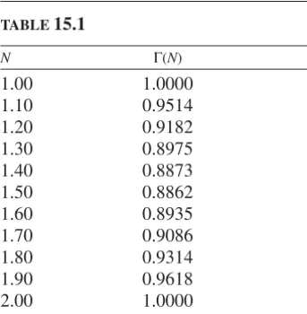
values in the interval 1 < x < 2 are known. (Any other interval of unit length will suffice.) Table 15.1 and the

graph in Figure 15.1 illustrate this idea.

Tables of Values and Graph of

the Gamma Function

TABLE 15.1

N Γ(N)

1.00 1.0000 1.10 0.9514 1.20 0.9182 1.30 0.8975 1.40 0.8873 1.50 0.8862 1.60 0.8935 1.70 0.9086 1.80 0.9314 1.90 0.9618 2.00 1.0000

Equation (2) is a recurrence relationship that leads to the factorial concept. First observe that if x = 1, then Equation (1) can be evaluated and in particular,

Γ(1) = 1

If the recurrence relation (2) is characterized as a differential equation, then the definition of Γ(x) can be

extended to negative real numbers by a process called analytic continuation. The key idea is that even though

Γ(x) as defined in Equation (1) is not convergent for x < 0, the relation ( )x 1 (x 1)

x

Γ = Γ + allows the meaning

to be extended to the interval – 1 < x < 0, and from there to – 2 < x < – 1, and so on. A general development

of this concept is beyond the scope of this presentation; however, some information is presented in Problem 15.7.

The factorial notion guides us to information about Γ(x + 1) in more than one way. In the eighteenth

cen-tury, James Stirling introduced the formula (for positive integer values n)

1

This is called Stirling’s formula, and it indicates that n!asymptotically approaches 1

2 n n

n e

π + − _{for large}

values of n. This information has proved useful, since n! is difficult to calculate for large values of n.

There is another consequence of Stirling’s formula. It suggests the possibility that for sufficiently large

values of x,

1

( 1) 2 x x

x! = Γ + ≈x π x +e− (5a)

(An argument supporting this is made in Problem 15.20.)

It is known that Γ(x + 1) satisfies the inequality

Sincen is fixed, the second limit is one; therefore, lim .

( 1) ( )

This factorial representation for positive integers suggests the possibility that

( 1) lim 1, 2,

Carl Friedrich Gauss verified this identification back in the nineteenth century.

This infinite product is symbolized by Π(x,k); i.e., Π(x,k) .

and through this symbolism,

( 1) lim ( , )

k

x x k

→∞

The expression for 1 ( )x

Γ [which has some advantage in developing the derivative of Γ(x)] results as

fol-lows. Put Equation (6) in the form

1 1

is Euler’s constant. This constant has been calculated to many places, a few of which are

γ ≈ 0.57721566 . . . .

Another result of special interest emanates from a comparison of Γ(x)Γ(1 – x) with the well-known

for-mula

[SeeDifferential and Integral Calculus, by R. Courant (translated by E. J. McShane), Blackie & Son Limited.]

Γ(1 – x) is obtained from ( )y 1 (y 1)

Now use Equation (8) to produce

Γ(x)Γ(1 – x) = 1 1 /

Observe that Equation (11a) yields the result 1

Theduplication formula

is also part of the literature. Its proof is given in Problem 15.24.

The duplication formula is a special case (m = 2) of the following product formula:

1

It can be shown that the gamma function has continuous derivatives of all orders. They are obtained by differentiating (with respect to the parameter) under the integral sign.

It helps to recall that 1 x-1

This result can be obtained (after making assumptions about the interchange of differentiation with limits) by taking the logarithm of both sides of Equation (9) and then differentiating.

In particular,

Γ′ (1) = –γ (γ is Euler’s constant.) (14b)

It also may be shown that

( ) 1 1 1 1

(See Problem 15.73 for further information.)

The Beta Function

The beta function is a two-parameter composition of gamma functions that has been useful enough in ap-plication to gain its own name. Its definition is

1 _{1 1}

It is shown in Problem 15.11 that the beta function can be expressed through gamma functions in the fol-lowing way

Many integrals can be expressed through beta and gamma functions. Two of special interest are

/ 2

Dirichlet Integrals

IfV denotes the closed region in the first octant bounded by the surface 1

p q r

coordinate planes, then if all the constants are positive,

1 1 1

Integrals of this type are called Dirichlet integrals and are often useful in evaluating multiple integrals

(see Problem 15.21).

15.2. _{Evaluate each of the following:}

(a) (6) 5! 5 4 3 2 30

(5.5) (4.5)(3.5)(2.5)(1.5)(0.5) (0.5) 315

Γ Γ Γ

15.3. _{Evaluate each integral.}

Let 2x = 7. Then the integral becomes

using Problem 12.31. This result also is described in Equation (11a, b) on Page 391.

15.5. _{Evaluate each integral.}

15.8. _{Prove that} x dx n

∫

this last integral becomes

1 1 1

Compare with Problem 8.50.

15.9. _{A particle is attracted toward a fixed point} O with a force inversely proportional to its instantaneous distance fromO. If the particle is released from rest, find the time for it to reach O

At time t = 0, let the particle be located on the x axis at x = a > 0 and let O be the origin. Then, by

wherem is the mass of the particle and k > 0 is a constant of proportionality.

Let dx

Similarly, 2 1 2

using the results of Problem 15.10. Hence, the required result follows.

This argument can be made rigorous by using a limiting procedure as in Problem 12.31.

15.12. _{Evaluate each of the following integrals.}

(a) 1 4 3

Letting x = 2υ, the integral becomes

2

This follows at once from Problems 15.10 and 15.11.

15.15. _Prove / 2 / 2

L is an even positive integer and

(b) 2 4 6 ( 1)

⋅ ⋅ [compare Problem 15.14(a)].

(b) The integral equals

/ 2 / 2 / 2

The method of Problem 15.14(b) can also be used.

(c) The given integral equals

/ 2

+ − the given integral becomes 1

and the result follows.

15.18. _Evaluate

15.19. _{Show that} 2 3 3

By definition, 1

0

To this point the analysis has been rigorous. The following formal steps can be made rigorous by incor-porating appropriate limiting procedures; however, because of the difficulty of the proofs, they have been omitted.

In Equation (2) introduce the logarithmic expansion

l

Whenx is replaced by integer values n, then the Stirling relation

! ( 1) 2 x x

n = Γ + ≈x πx x e− (5)

is obtained.

It is of interest that from Equation (4) we can also obtain the result (12) on Page 391. See Problem 15.72.

Dirichlet integrals

15.21. _Evaluate 1 1 y1

V

I=

∫∫∫

xα−yβ−z −dx dy dz, where V is the region in the first octant bounded by the sphere x2 _{+ y}2

Letx2 _{= u, y}2 _{= υ,z}2 _{= w. Then}

so that Equation (2) becomes

1

The integral evaluated here is a special case of the Dirichlet integral Equation (20), Page 393. The general case can be evaluated similarly.

15.24. _{Prove the} duplication formula 22p–1_{Γ(p)Γ(p +} 1

and the required result follows. (See Problem 15.74, where the duplication formula is developed for the simpler case of integers.)

as in Problem 15.23.

But / 2 / 2 / 2

Lettingu2 _{= υ in the last integral, we have, by Problem 15.17,}

Substitution of Equation (2) in Equation (1) yields the required result.

15.27. _Evaluate 2

This integral and the corresponding one for the sine [see Problem 15.68(a)] are called Fresnel integrals.

15.36. _{Prove that if m is a positive integer,} 1 ( 1) 2

Euler’s constant, as in Problem 11.49).

The beta function

9 3. [Hint: Differentiate with respect to Problem 15.46(b).]

15.48. _{Use the method of Problem 12.31 to justify the procedure used in Problem 15.11.}

Dirichlet integrals

15.49. _{Find the mass of the region in the} xy plane bounded by x + y = 1, x = 0, y = 0 if the density is σ =

xy

.

15.50. _{Find the mass of the region bounded by the ellipsoid} x

the distance from its center.

Ans.πabck

30 (a

2_+b2_+c2

),k= constant of proportionality

15.51. _{Find the volume of the region bounded by} x2/3 _{+ y}2/3 _{+ z}2/3 _{= 1.}

and choose r appropriately.)

15.63. _{Prove that for} m = 2, 3, 4, . . . , sinπ

, using Problem 15.63. (Hint: Take logarithms of the result in

Problem 15.63 and write the limit as m→⬁ as a definite integral.)

15.65. _{Prove that} Γ 1

L _{[Hint: Square the left-hand side and use}

Problem 15.63 and Equation (11a), Page 391.]

15.66. _{Prove that}

∫

_lnΓ_{( )}x dx=1_{In( ).}

15.72. _{Obtain Equation (12) on Page 391 from the result (4) of Problem 15.20. [Hint: Expand}

3_{/(3 n)}

e

υ

+

. . . in a power series and replace the lower limit of the integral by –⬁.]

15.73. _{Obtain the result (15) on Page 392. [Hint: Observe that}

( )

_x

1

(

_x

!)

Now take the logarithm of this expression and then differentiate. Also, recall the definition of the Euler constantγ.]

15.74. _{The duplication formula (13a), Page 392, is proved in Problem 15.24. For further insight, develop it for positive}

integers; i.e., show that 22n−1Γ n+1

350

We analyzed a simpler version of this problem in Example 1 of Section 3.2. Let be the amount of salt (in kilograms) in the tank at time t.Then of course is the concentration, in kilograms per liter. The salt content is depleted at the rate (6 L/min)

kg/min through the exit valve. Simultaneously, it is enriched through valves AandB at the rate given by

(1)

Thus, changes at a rate

or

(2) dx

dt 3

500xgAtB , d

dtxAtBgAtB 3xAtB

500 , xAtB

gAtB e0.4 kg/L

_{6 L/min2.4 kg/min , 0} 6 _t 6 _{10 (valve A) ,}

0.2 kg/L_{6 L/min1.2 kg/min , t} 7 _{10 (valve B) .}

gAtB, 3xAtB

_/

500

AxAtB

_/

1000 kg/ LB xAtB

_/

1000

xAtB

Laplace Transforms

INTRODUCTION: A MIXING PROBLEM

7.1

Figure 7.1 depicts a mixing problem with valved input feeders. At timet0, valve A is opened, delivering 6 L/min of a brine solution containing 0.4 kg of salt per liter. Att10 min, valveAis closed and valveBis opened, delivering 6 L/min of brine at a concentration of 0.2 kg/L. Initially, 30 kg of salt are dissolved in 1000 L of water in the tank. The exit valve C, which empties the tank at 6 L/min, main-tains the contents of the tank at constant volume. Assuming the solution is kept well stirred, determine the amount of salt in the tank at all timest_0.

x(t)

x(0)= 30 kg _{6 L/min} 1000 L

C

6 L/min, 0.4 kg/L

6 L/min, 0.2 kg/L

A

B

with initial condition

(3)

To solve the initial value problem (2)–(3) using the techniques of Chapter 4, we would have to break up the time interval into two subintervals (0, 10) and On these subintervals, the nonhomogeneous term is constant, and the method of undetermined coef-ficients could be applied to equation (2) to determine general solutions for each subinterval, each containing one arbitrary constant (in the associated homogeneous solutions). The initial condition (3) would fix this constant for but then we would need to evaluate

and use it to reset the constant in the general solution for

Our purpose here is to illustrate a new approach using Laplace transforms. As we will see, this method offers several advantages over the previous techniques. For one thing, it is much more convenient in solving initial value problems for linear constant coefficient equations when the forcing term contains jump discontinuities.

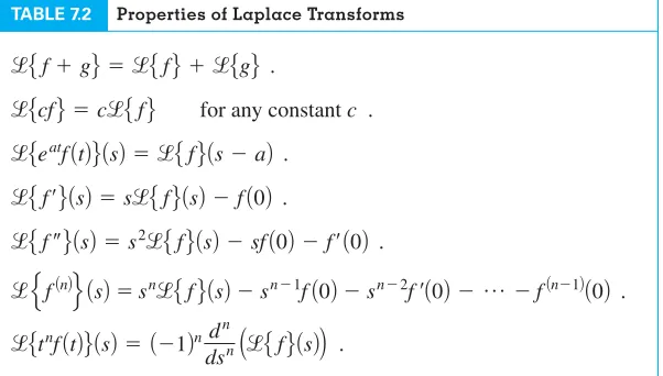
TheLaplace transformof a function defined on is given by†

(4)

Thus we multiply by and integrate with respect to tfrom 0 to This takes a function oftand produces a function of s.

In this chapter we’ll scrutinize many of the details on this “exchange of functions,” but for now let’s simply state the main advantage of executing the transform. The Laplace transform replaces linear constant coefficient differential equations in the t-domain by (simpler) alge-braic equations in the s-domain!In particular, if is the Laplace transform of then the transform of is simply Therefore, the information in the differential equa-tion (2) and initial condiequa-tion (3) is transformed from the t-domain to the s-domain simply as

t-Domain s-Domain

(5)

where is the Laplace transform of (Notice that we have taken certain linearity prop-erties for granted, such as the fact that the transform preserves sums and multiplications by constants.) We can find in the s-domain without solving any differential equations: the solution is simply

(6)

For this procedure to be useful, there has to be an easy way to convert from the t-domain to thes-domain and vice versa. There are, in fact, tables and theorems that facilitate this conver-sion in many useful circumstances. We’ll see, for instance, that the transform of g(t), despite its unpleasant piecewise specification in equation (1), is given by the single formula

and as a consequence the transform of equals XAsB 30

s₃

_/

₅₀₀

2.4 sAs₃

_/

₅₀₀B

1.2e10s sAs₃

_/

₅₀₀B . xAtB

GAsB 2.4 s

1.2 s e

₁₀s _,

XAsB 30 s₃

_/

₅₀₀

GAsB s₃

_/

₅₀₀ . XAsB

gAtB. GAsB

x¿AtB 3

500xAtBgAtB , xA0B30 ; sXAsB30 3

500XAsBGAsB , sXAsBxA0B.

x¿A_tB

xAtB, XAsB

q_.

est fAtB FAsBJ

q

0

estfAtBdt .

3

0,qB_,

fAtB,

t 7 _10.

xA10B

0 6 t 6 _10,

gAtB

A10,qB_.

A0,qB

xA0B_{30 .}

†_{Historical Footnote:The Laplace transform was first introduced by Pierre Laplace in 1779 in his research on}

Again by table lookup (and a little theory), we can deduce that

(7)

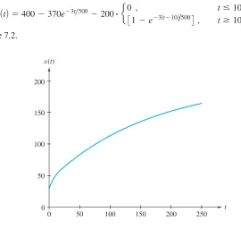
See Figure 7.2.

xAtB_400370e3t_/500₂₀₀

#

e0 , t10 ,

3

1e3At10B

/

500

4

, t_{10 .}

t x(t)

50 0

0 50 100 150 200

100 150 200 250

Figure 7.2 Solution to mixing tank example

Note that to arrive at (7) we did not have to take derivatives of trial solutions, break up intervals, or evaluate constants through initial data. The Laplace transform machinery replaces all of these operations by basic algebra: addition, subtraction, multiplication, division—and, of course, the judicious use of the table. Figure 7.3 depicts the advantages of the transform method. Unfortunately, the Laplace transform method is less helpful with equations containing variable coefficients or nonlinear equations (and sometimes determining inverse transforms can be a Herculean task!). But it is ideally suited for many problems arising in applications. Thus, we devote the present chapter to this important topic.

Differential equation

Inverse transform Laplace

transform

Break into subintervals

Trial solutions

Solution

Algebra:+,−,× ,÷ ,∫dt

Calculus:

Fit constants to initial data

t- domain

s-domain

d dt