teach about feedback in physics
Michael Lingard
Grenville College, Bideford, Devon, UK
Abstract
This article looks generally at spreadsheet modelling of feedback situations.
It has several benefits as a teaching tool. Additionally, a consideration of the
limitations of calculating at many discrete points can lead, at A-level, to an
appreciation of the need for the calculus. Feedback situations can be used to
introduce the idea of differential equations. Microsoft Excel
™is the
spreadsheet used.
Introduction
Situations involving feedback abound in physics. They are commonly expressed mathematically as differential equations in which the rate of change of a quantity is a function of that quantity. They can occur in situations involving feedback loops (both positive and negative feedback). Two examples are as follows:
• radioactive decay (dN/dt = −λN, whereN
is the number of nuclei present andλis the probability per unit time of decay, known as the decay constant). Here the differential equation represents the feedback loop:
“the activity (dN/dt) causes a decrease inN, which causes a decrease in activity, which causes a smaller decrease inN, which causes…”
• a body falling in the presence of a drag force
(Newton’s second law gives
mv=(mg−kv2)t, wherevis the
velocity of an object of massm,kis a ‘drag coefficient’ andkv2is the drag force). The
feedback loop corresponding to this is the familiar terminal velocity case—see the Frontline article on page 383 of this issue.
Severn (1999) uses spreadsheet modelling to provide solutions to such differential equations.
For example, by using suitably small time intervals, the equation mv = (mg−kv2)t
can be used to calculate successive values of v over time. The treatment of terminal velocity also uses iterative processes on a spreadsheet, but I use themat each stage in the feedback loop, instead of on the fully formed differential equation. This confers the following four benefits:
• younger students who have no understanding
of differential equations can produce solutions to them, using very basic physics (in the terminal velocity example, very little more thanF =mais required).
• the variation with time of all parameters in
the equation can be investigated (in the terminal velocity example acceleration–time graphs can be formed as well as
velocity–time graphs).
• causal relationships and the nature of the
feedback loop become apparent from the spreadsheet in a more explicit way than from a fully formed differential equation.
• the spreadsheet shows up the shortcomings
of the numerical modelling more explicitly, which helps to explain the usefulness of the calculus.
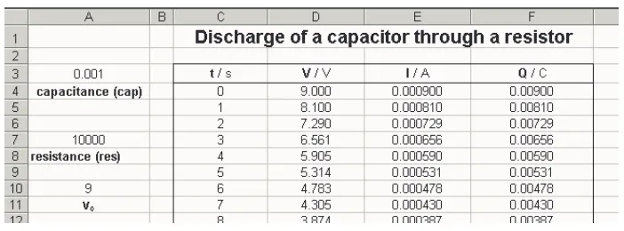
Figure 1.The first few lines of formulae modelling the discharge of a 1000µF capacitor through a 10 kresistor.
Figure 2.The first few lines of calculated data modelling the discharge of a 1000µF capacitor through a 10 k
resistor.
Younger students gain access to physics
that would usually be beyond them
mathematically
ApplyingF =mato the case of a falling body in
air givesmv=(mg−kv2)t, wheremgis the
weight andkv2 is the drag. Thereforemg
−kv2
is simply the resultant force, and acceleration has been written asv/t.
A typical 14-year-old in the UK would not be expected to solve an equation such as this, and yet we have seen in the Frontline article that (s)he can perform sophisticated quantitative work using spreadsheet modelling and produce what amounts to a graphical solution of this equation.
More than one variable can be modelled
at a time
In the terminal velocity example above:
“the velocity is calculated from the
acceleration, which comes from the resultant force, which comes from the drag, which comes from the velocity …”
This means that the time dependence of any of these quantities can be observed immediately
from the appropriate column of the table, or by constructing a separate graph. We have already seen that variations in the acceleration can be linked to the changing gradient of the velocity– time graph.
Another example is the modelling of capacitor discharge through a resistor. The spreadsheet given is for a 1000 µF capacitor and a 10 k resistor. Figures 1 and 2 show the first few lines of formulae and calculated data, respectively, while figure 3 is the graph showing the decay of potential difference across the capacitor.
The spreadsheet is easy for A-level students to construct, because the only physics required are the formulae Q = CV andV = I R. The
exponential discharge formula Q = Q0e−t /CR
is not required, and thus students can appreciate where exponential relationships in physics come from. The trick (which makes the feedback appear) is to realize that (since the time intervals, t, are equal to 1 s and I = Q/t) each
charge value is equal tothe previous one minus the appropriate current.
potential dif
Figure 3.The decay of potential difference across a capacitor.
construct graphs of charge stored against time, or current against time. In this way, the student can appreciate that all three ofV,I andQdecay exponentially.
A affects B affects C affects A. . .
Because each variable has a column of its own in the spreadsheet, and each column is calculated from at least one other, it is easy to see the causal relationships within the feedback loops. We have already seen that, in the terminal velocity example:
“the velocity is calculated from the acceleration column, which comes from the resultant force column, which comes from the drag column, which comes from the velocity column. . . ”
Many students will gain more insight from this into the physics of the situation than they will from forming a single differential equation and then solving it.
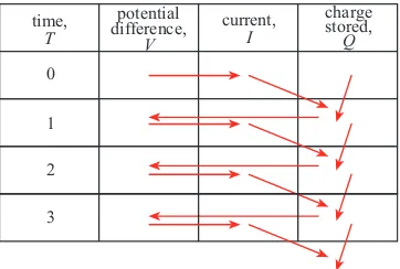
I like my students to express these relation-ships diagrammatically, using arrows on a blank copy of the spreadsheet. For example, if A→ B
means ‘B is calculated from A’, then the iterative calculations on the terminal velocity spreadsheet could be represented as shown in figure 4. This diagrammatic representation makes it easy to see which variables affect which others, and the repeating pattern makes clear the nature of the feedback loop.
The feedback loop that leads to the exponen-tial discharge of a capacitor can be written as:
“The initial potential difference determines the current, which changes the charge stored, which changes the potential difference, which changes. . . ”
Figure 4.Representation of the calculations on the terminal velocity spreadsheet.
Figure 5.Representation of the exponential discharge of a capacitor.
The diagrammatic representation of this feedback loop is shown in figure 5.
Note that the differential equations modelled in this article all deal with rates of change with respect to time, but this modelling technique will work for all feedback situations. The easier the physics at each step of the feedback loop, the more accessible the situation will be to students. Complicated overall pictures (see, for example, mv = (mg−kv2)t, whichiscomplicated if
you are a British 16-year-old!) can be broken down into a series of easy steps. In my opinion, once the student is used to working with spreadsheets, the modelling is then only as hard as the hardest single step.
All the models in this article have in common that the next value is calculated by adding (or subtracting) a rate of change to aprevious value. For example,
v(t )=v(t−1)+acceleration
in the model of terminal velocity,
Q(t )=Q(t−1)−current
in the capacitor discharge model.
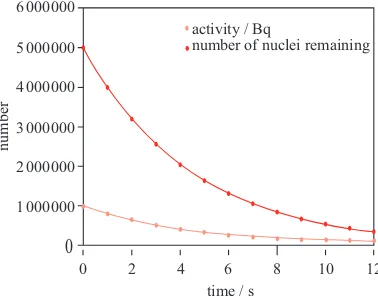
Figure 6.The first few lines of formulae for the decay of 5 million atoms withλ=0.2 s−1.
Figure 7.The first few lines of calculated data for the decay of 5 million atoms withλ=0.2 s−1.
will be needed. More advanced students may well see the connection between these relationships and the calculus, but unfortunately this has not yet happened in my classes!
Models can be mathematically incorrect!
In the terminology of the previous section, we can set up a model of radioactive decay (in fact, it is the most straightforward of the three models presented here) by using the number of nuclei to calculate the activity to calculate the number of nuclei to calculate the activity. . . etc, i.e.
N (t )=N (t−1)−A(t−1)
and A(t ) = λN (t ) where A = dN/dt is the
activity of the sample.
Figures 6, 7 and 8 show the spreadsheets and graph for the radioactive decay of 5 million atoms of an isotope whose decay constant,λ, is equal to 0.2 s−1. In other words, each nucleus has a 1 in 5 chance of decaying each second. The INT function has been used to round off numbers to integer values, in recognition of the fact that fractions of an atom are meaningless.
Notice that the number of nuclei and the activity can both be modelled on the same graph, and that the nature of the feedback is clear from the table. Diagrammatically the feedback loop looks as shown in figure 9. The simplicity of
number
time / s
0 2 4 6 8 10
0
12 6 000 000
5 000 000
4 000 000
3 000 000
2 000 000
1 000 000
activity / Bq
number of nuclei remaining
Figure 8.The radioactive decay of 5 million atoms withλ=0.2 s−1.
the feedback diagram reflects the comparative simplicity of setting up this particular spreadsheet. At first sight, it looks like the graph shows a nice exponential function. We are told that exponential functions result when the rate of change of a quantity is proportional to that quantity, and it looks as though that is the case here, since the activity at each time is found by multiplying the number of nuclei by a constant fraction (the decay constant).
2
3
Figure 9.Feedback diagram for radioactive decay.
number of nuclei remaining
time / s
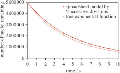
Figure 10.Comparison of the original model and the true exponential function.
be seen in figure 10, in which the original model is plotted alongside the true exponential function N =N0e−0.2t. The model has values of number
of nuclei remaining that are too low (another way of saying this is that the model overestimates the activity).
Why is this? Why does our model not provide a true exponential function? Well, our model calculates an activity from the number of nuclei, and it does it very well, but it applies this activityfor the whole second, until the next row of the spreadsheet, when it recalculates. In reality, the activity changes not in discrete steps, but continually. In each interval of one second the activity will be falling, whereas our model assumes it to stay at its initial value. This leads our model to overestimate the activity at each step, and to underestimate the number of nuclei remaining. (As an aside, for this reason those of you who throw ‘Anderson cubes’ to model radioactive decay should expect a better fit to our spreadsheet model than to the true exponential function!)
The student should see easily from this that using smaller time intervals, δt, should give a
This exercise thus shows the student that a model is just that—only a model, and it can help students to see why the calculus is so useful and how it comes about.
The difference between the model and the true exponential function can be seen mathematically. Each value ofNin the model is just four-fifths (1−
λ) of the previous value. ThusN =N0(1−λ)t.
A-level students with good mathematical skills could be given the task of expanding this function binomially and comparing it with a power series expansion ofN =N0e−λt.
Conclusion
Spreadsheets can be used to model physical situ-ations involving feedback loops, and thus provide graphical solutions to differential equations. Parameters can easily be changed and their effects investigated. The causal relationships that cause the feedback loop become apparent in the spreadsheet model and it can be instructive for the student to make them explicit in diagram-matic form. The student can benefit from con-sidering the mathematical limitations of the model. Spreadsheet modelling can help the student understand feedback situations without having to learn differential equations, and therefore the student can learn certain areas of physics quantitatively at a younger age than would otherwise be the case.
Received 15 January 2003, in final form 16 May 2003 PII: S0031-9120(03)58327-7
Reference
Severn J 1999 Use of spreadsheets for demonstrating the solutions of simple differential equations
Phys. Educ.34360–6
Michael Lingardis Head of Physics and