Technology and Economics
&
University of New Hampshire
BSc FINAL PROJECT
Investigation of Continuous
Nonlinear Systems
László Péter Kindrat
Department of Automation and Applied Informatics
Group of Electrical Engineering
Supervisor:
Péter Stumpf
Acceptable (signature, date):
Department of Electrical and Computer Engineering
Budapest University of Technology and Economics Faculty of Electrical Engineering and Informatics Department of Automation and Applied Informatics
Group of Electrical Engineering
Magyar tudósok krt 2. QB108. 1117Budapest,
Hungary
Phone: +36-1-463-1165, Fax: +36-1-463-3163 Web: http://www.get.bme.hu
E-mail: info@get.bme.hu
FINAL PROJECT (BSc)
SZD /2013
Title: Investigation of Continuous Nonlinear Systems
Assigned to: (Neptun code): László Péter KINDRAT (IJHRRD)
Phone: +36-70-2518951 , e-mail: laszlokindrat@gmail.com
Course / Specialization: BSC in Mechatronics Engineering / Integrated Engineering
Supervisor(s): Péter Stumpf
Department of Automation and Applied Informatics Budapest University of Technology and Economics Phone: +36-1-463-2337, E-mail: stumpf@get.bme.hu
Allen D. Drake
Electrical and Computer Engineering Department University of New Hampshire
Phone: +1-603-862-1325, E-mail: allen.drake@unh.edu
Subjects of the final exam (code):
1. Mechatronika
Mechatronika I. (BMEGEFOAMM1) Mechatronika II. (BMEGEFOAMM2) 2. Analóg és digitális technika
Analóg elektronika (BMEVIAUA009) Digitális elektronika (BMEVIAUA010) 3. Power Motion Control
Power Electronics (BMEVIAUA017) Motion Control (BMEVIAUA016)
Date of issue / submission: August 26, 2013 / December 17, 2013
General Requirements:
1. The students are expected to have regular contact with their supervisor(s) at least once in a week. The
Attendance Check Sheet (ACS) must be signed by the supervisor in each consultation. ACS must be attached to the Final Project.
2. One page working plan (description and schedule of tasks) has to be submitted by week 5.
3. The Final Project has to be submitted electronically in a CD ROM and in one hard copy by the deadline. For the
details of formal requirements see the guideline in the document HOW TO PREPARE YOUR FINAL PROJECT
found in the web pages of the Group of Electrical Engineering (www.get.bme.hu).
4. Before submitting the Project, the hard copy should be endorsed by the Supervisor(s).
5. The Final Project has to include a short review of the technical publications in the field of the project. Any
information taken from the technical literature or other sources has to clearly be identified.
6. The Final Project must contain the sheet entitled: ”Declaration” signed by the student and the current sheet, the assignment. The Declaration is included in the document guideline/template.
7. The preparation of an A2 size poster summarizing the project is required. It must be submitted only
electronically in the CD-ROM.
8. The oral presentations of the results of the Final Projects will in the final examination. Usage of Computer
Projector is compulsory.
9. Failing to meet the requirements listed above might result in the rejection of granting mark and credit assigned
to the Final project.
Budapest University of Technology and Economics Faculty of Electrical Engineering and Informatics Department of Automation and Applied Informatics
Group of Electrical Engineering
Magyar tudósok krt 2. QB108. 1117Budapest,
Hungary
Phone: +36-1-463-1165, Fax: +36-1-463-3163 Web: http://www.get.bme.hu
E-mail: info@get.bme.hu
Task outline: The modern theory of nonlinear dynamics and specially the chaos
theory, although is admittedly still young, has spread like wild fire into all branches of science. Therefore the demonstration of nonlinear
behaviour and chaotic phenomena is an important part of an engineer’s
education.
The aim of the project is to get familiar with the theory of nonlinear dynamics and chaos. Investigate a few nonlinear systems (e.g. Van der Pol, Lorenz, Duffing, etc.) by simulation and analytic calculation. Implement these systems on circuit board and examine their behaviour.
The final goal of the project is to design a printed circuit board, which would serve as a demonstrational tool for nonlinear and chaotic systems.
Tasks in detail: 1. Study the technical literature of the theory of nonlinear dynamics
and chaos
2. Investigate nonlinear ordinary differential equation systems by
numerical and analytical methods
3. Implement these systems on circuit board, conduct measurements
and compare with simulation results
4. Design a PCB on which students can implement various nonlinear
systems and can study their behaviour
Budapest, September , 2013
………. Prof. Dr. István Vajk, Head
Department of Automation and Applied Informatics
I approve the project:
Budapest, September , 2013
……….
Prof. Dr. Tibor Czigány
Dean of Mechanical Engineering
I hereby confirm that I fulfilled all prerequisites of the final project. If not, I take notice of loosing the availability of the above proposal.
Budapest,
……… student
………….
I, the undersigned László Péter Kindrat, hereby declare that the Final Project submitted contains the results of my own work, assisted by my supervisors and that all other results taken from the technical literature or other sources are clearly identified and referred to. I accept that the results presented in my Final Project can be utilized by the Departments of the supervisors for further research or teach-ing purposes.
Budapest, January 4, 2014
signature
This paper consists of four main parts. The first part is covered in Chapter 1, and summarizes the goals of the project. The second part includes a historical and mathematical introduction to the topic of nonlinear dynamics and chaos theory. This is covered in Chapter2. The third part is the analytical and numerical inves-tigation of two specific nonlinear systems, namely the Van der Pol equation and the Lorenz system. In the fourth part the design and testing of a demonstrational circuit board is discussed.
In the mathematical background, firstly the ordinary differential equations are introduced, followed by the concept of phase space, and Poincaré mapping. The tools for the investigation of dynamical systems are further described by intro-ducing the linear stability analysis, and classifying equilibrium points in two and three dimensions. That is followed by the description of closed curves in the phase portrait, specifically limit cycles, homoclinic orbits, heteroclinic connections, frequency-locked states and quasi-periodic oscillations. In the last section of this chapter, the deterministic chaos is described. For this, the concept bifurcation diagram, the Feigenbaum constants and Lyapunov exponent are introduced.
In Chapter 3 the equilibrium points of the Van der Pol oscillator are analyzed first. Then the limit cycle is described, along with the analysis of the bifurcation diagram of the autonomous system. As a conclusion of the chapter, the forced equation is analyzed by numerical methods, including the simulation of a bifurca-tion diagram and frequency analysis of the solubifurca-tions. Chapter 4 starts with the investigation of the stable solutions of the system. Then the strange attractor is described. The attractor’s behavior as a function of its parameter values is examined too.
The third main part will start by explaining the methods used for the analog circuit implementation of differential equations. It is followed by the description of a printed circuit board designed for such implementations. Chapter5concludes with the short evaluation of the built board.
The paper is closed by a short conclusion and an overview of the possible continuations of the paper.
E szakdolgozat tematikailag négy fő részből áll. Az első rész a projekt cél-jait foglalja össze és az 1. fejezet foglalja magában. A második rész történeti és matematikai bevezetés a nemlineáris dinamikai és káoszelmélet témakörébe, melyet a 2. fejezet tartalmaz. A harmadik részben a Van der Pol oszcillátor és a Lorenz egyenlet analitikus és szimulációs módszerekkel történő vizsgálatának leírása történik. A negyedik részben egy demonstrációs nyomtatott áramkör ter-vezésének és tesztelésének leírása található.
A matematikai háttér leírása a hagyományos differenciálegyenletek bevezetésével kezdődik, melyet a fázistér leírás és a Poincaré-metszet bemutatása követ. További dinamikai rendszerek vizsgálatára szolgáló eszközök bemutatására is sor kerül, úgy mint a spektrális stabilitásvizsgálat, egyensúlyi pontok és osztályozásuk két és három dimenzióban, valamint a fázisportrén található zárt görbék osztályozása (hetero- és homoklinikus kapcsolatok, határciklusok, kváziperiodikus és frekven-cia zárt hurkok). E fejezet utolsó szakaszában a determinisztikus káosz leírása történik, melyhez bevezetésre kerülnek a bifurkációs diagram, a Feigenbaum-állandók és a Ljapunov-exponens fogalmak.
A 3. fejezet a gerjesztetlen Van der Pol oszcillátor egyensúlyi megoldásainak vizsgálatával indul. Ezután a határciklus leírása történik, a bifurkációs diagram vizsgálatával kiegészítve. A fejezet második felében a gerjesztett egyenlet vizs-gálata történik numerikus módszerekkel, a bifurkációs diagram és a frekvencia spektrum segítségével. A 4. fejezetet szintén a fixpontok vizsgálatával kezdődik, melyet a különös attraktor leírása követ. Az attraktor vizsgálata a paraméter értékek függvényében szintén sorra kerül.
A dolgozat harmadik tematikai egysége (5. fejezet) a differenciál egyenletek analóg áramköri megvalósításának hátterével indul. Ezt követően egy demon-strációs célokra tervezett nyomtatott áramköri lap tervezésének leírása történik, melyet a megépített eszköz rövid (mérésekkel történő) vizsgálata követ.
A dolgozatot rövid összefoglalás és a lehetséges folytatásra való kitekintés zárja.
I would like to thank my advisors Allen D. Drake (University of New Hampshire) and Péter Stumpf (Budapest University of Technology and Economics) for their help and guidance during my work. I would also like to thank Prof. Nicholas Kirsch (University of New Hampshire) for taking the time to help me with the milling of the printed circuit board.
Moreover, I would like to express my gratitude for NI Hungary Kft., and es-pecially for Balázs Daróczi for helping me with my project during my summer internship and supplying me with electrical components for my measurements.
At last, but not least I want to thank the staff of both the Budapest University of Technology and Economics and the University of New Hampshire for making my semester abroad possible.
Task outline i
Declaration iii
Abstract iv
Kivonat v
Acknowledgments vi
Contents vii
1 Introduction 1
1.1 Goals. . . 1
1.2 Historical and mathematical background . . . 2
1.3 Investigation of specific nonlinear systems . . . 2
1.4 Demonstrational printed circuit board . . . 4
2 Background 6 2.1 Ordinary differential equations . . . 7
2.2 Phase space . . . 9
2.3 Poincaré concept . . . 13
2.4 Equilibrium points . . . 16
2.5 Closed trajectories . . . 23
2.6 Quasi-periodic oscillations and frequency-locked loops . . . 27
2.7 Chaotic state . . . 29
3 The Van der Pol oscillator 35 3.1 Fixed points . . . 35
3.2 Limit cycle . . . 37
3.3 External forcing . . . 39
4 The Lorenz system 41 4.1 Fixed points . . . 42
4.2 Strange attractor . . . 43
5 Demonstrational printed circuit board 45
5.1 Implementing differential equations as analog circuits . . . 45
5.2 Design of the circuit board . . . 49
5.3 Building the circuit board . . . 51
5.4 Testing the circuit board . . . 53
6 Conclusions and continuation of the project 54 A Implementation of specific equations as analog circuits 56 A.1 Implementing 5.6 in NI Multisim . . . 56
B Schematics and pictures of the PCB 63
C Large figures of simulated systems 69
Introduction
The origins of chaos theory lead back to the end of 19th century. It started to become a popular field of research among mathematicians in the 1960s, which makes it a relatively young area of science. Although it has been getting seri-ous attention among mathematicians, its applications in engineering still hold a great potential and offer a wide range of practical research topics, generating an enormous body of literature worldwide.
To cover the topic to the extent necessary for a bachelor’s level final project, my paper will cover multiple, reasonably simple aspects. I will use a purely analytical approach, along with numerical methods to discuss chaotic phenomena in theory. For a conclusion, I will design a prototyping board, which will act as an optimized tool for the measurement of the electronic implementation of such systems.
1.1
Goals
My first goal is to gather and process extensive literature on the topic of chaos and nonlinear dynamics. As I have had an interest in this topic for some time, I already have become familiar with a part of this subject. Also, I have been studying the mathematical concepts surrounding differential equations, stability, and chaos.
Secondly, I intend to make this project beneficial for not only myself, but for other students and possibly for academic staff, too. In order to achieve this, the project will include the design and testing of a printed circuit board for the demonstration of nonlinear dynamics and chaotic phenomena. In order to achieve this goal I will extend my knowledge in the area of PCB design, more specifically in the use of the Altium Designer.
Thirdly, as this project will be the most significant project of my academic career so far, I will need to manage this project well. This will require me to improve my time management skills and to prioritize my tasks and goals.
Furthermore, I plan to write the documentation in LATEX. This will require some
extra effort, but because I plan to use mathematical formulations and notations, the better look will definitely be worth the time. For some of the illustrations, I will use Inkscape, an Open Source vector graphics editor, which I will get acquainted with on the way.
1.2
Historical and mathematical background
I plan to start my thesis with a brief historical introduction to the topic. Along with this short summary, I will introduce some of the concepts which were defined in the early days of this new field of science and are still used. Later on, I will define these concepts after classifying differential equations in order to specify the type of differential equations I am going to deal with later in my paper. I will also include the definitions of a few concepts used in the study of ordinary differential equations, namely the interpretation of phase space, definition and classification of equilibrium points and limit cycles in 2- and 3-dimensional phase space. Clarifying these will let me explain the basics of stability analysis, the concept of the Lyapunov-exponent and the Poincaré-section. I will define and describe attractors and the so-called basins of attraction, leading to the idea of chaos.
Later on I will give explanatory answers to the most obvious questions arising from nonlinear dynamics: “What is chaos? Where does it occur? What does non-linearity mean?” Spectacular examples of chaotic behavior (e.g Rössler attractor) will be given in this chapter in order to show the wide area of possible applica-tions. I will stress the connection between order and chaos, as it is discussed in the modern study of chaos theory. I will clarify the meaning of determination and the difference between “ordinary,” deterministically chaotic systems and the “real randomness” occurring in quantum-level systems.
1.3
Investigation of specific nonlinear systems
of chaotic and nonlinear behavior.
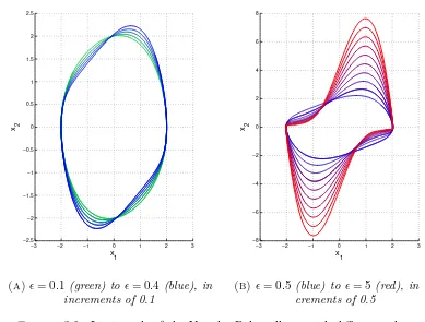
The first equation of interest is the so-called Van der Pol oscillator. The system was named after its first researcher, Dutch physicist Balthazar van der Pol. The system describes a second-order oscillator with nonlinear damping[1]:
¨
u−ǫ(α−u2) ˙u+u= 0
where ǫ and α are parameters and u is a function of time.
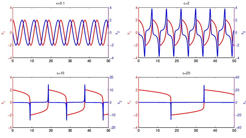
This oscillator produces so called relaxation-oscillations (as Van der Pol named them), in mathematics known as limit cycles, which was one of the first typical marks of nonlinear behavior to be identified. It is called an oscillator, because without excitation the system acts as a function generator with a distinct wave-form. When a sinusoidal forcing term is introduced, the system starts to produce irregular output signals as we go near its natural frequencies. Van der Pol found this in 1927, discovering one of the first examples of what was later called deter-ministic chaos.
The second system I would like to examine is the Lorenz-system. The system of equations was first derived by and named after Edward Lorenz, one of the founders of chaos theory studies. He derived the equations from a meteorological convection model he was studying. This is a third-order, nonlinear differential equation that can be written in the following form[2]:
˙
x=−σx+σy
˙
y=−xz+ρx−y
˙
z=xy−βz
where x, y and z are the state variables andσ, ρand β are parameters.
In my thesis I would like to approach these equations with different methods. Solutions for nonlinear differential equations can rarely be expressed in an explicit form, which is the case here. On the other hand, some analytical results are available for both above mentioned equations. I will attempt to do a few selected analytic calculation and cite other interesting results, which point beyond this paper.
Where analytical methods fail, numerical methods can still be used. In the study of nonlinear dynamics, these methods are often the only tool for examina-tion and definitely the most convenient method for an engineer. For each equa-tion, I will use Matlab simulations, which will produce graphical representations of behavior in time and frequency domain and also in state-space. Due to the sensitivity to differences in initial value, numerical modeling of nonlinear systems can be tricky, as improperly chosen values of method parameters such as time step size, can lead to nonsense or deceptive results.
1.4
Demonstrational printed circuit board
The final part of my project will be the design of a printed circuit board. My main concept is an electronic hardware sandbox specialized in a way that it could be effectively used to demonstrate the operation of analog computers and through this, the behavior of nonlinear systems.
First, the board will include operational amplifiers. These are the main com-ponents of an analog computer, as these are the building blocks of integrators. Op-amps can also be used for other linear operations, such as summation, divid-ing and scaldivid-ing signals. Furthermore, they can be used to implement a variety of nonlinear elements, such as resistors with negative or piece-wise linear character-istics and many others.
Secondly, the board will include linear-passive elements, mainly capacitors and resistors. The capacitors are needed for the integrators while the resistors are necessary for adjusting the time-constants and scaling. Some potentiometers will also be put on the board, to allow for manual control of parameters.
Thirdly, digital potentiometers will allow the users to control parameters through a computer. This will allow computer-controlled measurement routines to be run, which will serve as a tool for studying the behavior of a system at different pa-rameter values.
voltage supply. This design would simplify the process of building a circuit, as there will be no errors from improper connection of supply and ground pins. Fur-thermore, as the top side is not crowded with elements, it will make it easier to scan complicated circuits for debugging.
Placing digital and manually controlled potentiometers will allow this board to be used with simple lab equipment (DC voltage supply, function generator, scope). It also can be used with a computer controlled, fully automatic measurement system.
For the testing of the board, I will use a Digilent Electronics Explorer Board (EE Board), as the Department of Automation and Applied Informatics has sev-eral of these. This board features a 4-channel scope, 2 arbitrary (analog) function generators and a 32 channel digital I/O, along with programmable reference volt-ages and power supplies. These features will allow testing every feature of my PCB.
Background
The history of chaos theory starts with French scientist Henri Poincaré (1854-1912). He was one of the last mathematicians who contributed to all fields of mathematics, while his work as an engineer and physicist is also notable. This universality let him to lay down many vital concepts of what we call today applied mathematics. Among other highlights of his legacy, some of his results were crucial to the formulation of theory of relativity, and he was a pioneer of topology.
In 1886 Oscar II, King of Sweden, established a prize for mathematicians who could solve – among three other problems – what is called today the n-body problem. The original phrasing of the problem as stated in Acta Mathematica, vol. 7, of 1885-1886, was the following:
“Given a system of arbitrarily many mass points that attract each according to Newton’s law, under the assumption that no two points ever collide, try to find a representation of the coordinates of each point as a series in a variable that is some known function of time and for all of whose values the series converges uniformly.”
Poincaré won this prize with his article Sur le problème des trois corps et les
équations de la dynamiqueprinted later in 1890, in which he described some partial solutions for the three–body problem. Although he did not give a solution to the problem stated above, his 270 page article included fundamental results on the topic, and revealed that the problem was much more sophisticated than anyone suspected[4].
The work of Poincaré did not only consist of pure results, theorems and defini-tions. During his previous research he introduced a brand new methodology, which was based on the qualitative analysis of differential equations. Instead of trying to solve the equations analytically, he developed methods which let him examine the systems’ general behavior and its dynamics over time often using geometrical
tools. He used this pioneering approach successfully in his award-winning paper, which later served as an outline for a three volume book, Les méthodes nouvelles de la mécanique céleste(New Methods of Celestial Mechanics)[4]. While discussing his partial solutions for the three body problem, he designed the tools – of which I will also use a few later on – for a more general approach.
In the last volume of the series he described a strange phenomenon which he called a homoclinic tangle. This was the first encounter of what we call today deterministic chaos, making him the first person to discover a deterministic chaotic system. To understand some of Poincaré’s groundbreaking concepts, I will attempt to summarize some necessary mathematical concepts.
2.1
Ordinary differential equations
Letx∈Cn(U), U⊆R, andn∈N+whereCn(U) denotes the set of functions which
are k times continuously differentiable on U. Classically, an ordinary differential equation (ODE) is written as[5]:
F(t, x, x(1), x(2), . . . , x(n)) = 0 (2.1)
where F is continuous on a subset of Rn+2, and the order of the ODE is the
highest order derivative appearing in F. t∈U is the independent variable (often corresponding to physical time, hence the notation t), and for a k∈N+
x(k)(t) = d
kx(t)
dtk .
This general form is not very convenient for further analysis, so we will only consider equations in the form of
x(n)=f(t, x, x(1), x(2), . . . , x(n−1)
) (2.2)
which form can be derived from2.1at least locally, ifF has certain properties (see [5]). From now on – if not noted otherwise – we will consider the caset>0.
Extendingx to single-variable, vector-valued real functions,x:R→Rm, we get
a system of ordinary differential equations:
x(n)1 =f1(t,x,x(1),x(2), . . . ,x(n
−1)
) ...
x(n)m =fm(t,x,x(1),x(2), . . . ,x(n
−1)
)
Such system is called linear, if
x(n)i =gi(t) +
m
X
j=1 n−1
X
l=1
fi,j,l(t)x (l)
j . (2.4)
The system is called homogeneous, if gi(t)≡0.
A system of arbitrary order can always be rewritten as a system of first order equations. Using the substitution yj =x(j−1), j∈ {1,2, . . . , n}in 2.2, results in:
˙
y1=y2
... ˙
yn−1=yn
˙
yn=f(t, y1, . . . , yn)
(2.5)
In this case, the system is linear if f is linear in eachyj:
f(t, y1, . . . , yn) =g(t) +
n
X
j=1
aj(t)yj. (2.6)
It is sometimes written in the matrix form
˙ y1 ˙ y2 ... ˙
yn−1
˙ yn =
0 1 0 · · · 0
0 0 1 · · · 0
... ... ... . .. ...
0 0 0 · · · 1
a1(t) a2(t) a3(t) · · · an(t)
y1 y2
yn−1
yn + 0 0 ... 0
g(t)
. (2.7)
Similarly to2.7, ifg(t)≡0, the system is homogeneous, meaning that there is no excitation applied on the system. With other words, the system is homogeneous if
f does not contain terms which depend only on t or which are constants. In this sense, we can consider homogeneity for non-linear systems as well.
It is important to distinguish the concept of homogeneous systems from au-tonomous systems. An auau-tonomous system does not depend ontexplicitly, mean-ing that in 2.5 we have
˙
yn=f(y1, . . . , yn)
Admittingtas a new dependent variableyn+1=t,y˙n+1=1, any non-autonomous
getting an autonomous system will be the loss of linearity. On the other hand, we can (and later will) utilize this tool to simplify the analysis of nonlinear systems, and deal with excitations in a convenient way.
From now on, we will deal with systems whose structure do not depend on time and hence can be written as
˙
x=f(x) +g(t), (2.8) where x(t),g(t) :R→Rm,f(x) :Rm→Rm and f(x) is smooth. Because of this,
we can refer to homogeneous or unexcited systems as autonomous, and to forced equations as non-autonomous.
We consider ξ(t) a general solution of the system 2.8 if ξ˙(t) =f(ξ(t)) +g(t) applies. It is general, because such solution has free parameters, defining a family of functions instead of one particular function. By introducing the initial state
x(0) =x0, we can choose a particular function from this family. Therefore ξ(t) is
a particular solution, if it solves the initial value problem (IVP)
˙
x(t) =f(x(t)) +g(t), x(0) =x0. (2.9)
2.2
Phase space
The state of an autonomous system
˙
x=f(x), (2.10)
at a given timet is defined by its state vectorx(t), meaning that we can represent each distinct state by a single point in an m-dimensional Euclidean space. Each coordinate axis in such system measures the value of one single state variable xi,
thus corresponding to one degree of freedom.
As the system’s state evolves in time, the distinct points representing the ac-quired states describe a path in the m-dimensional space, which is called a tra-jectory (or phase curve). In other words, a tratra-jectory represents a set of states evolved from one particular initial statex0, hence being a particular solution to the
initial value problem. For a given autonomous system the trajectories depend only on the initial state and time, so they can be expressed as a functionx= Φ(x0, t),
−0.5 0 0.5 1 −1 −0.8 −0.6 −0.4 −0.2 0 0.2 0.4 0.6 x1 x2
−2 −1 0 1 2
−1 −0.5 0 0.5 1 x1 x2
−3 −2 −1 0 1 2 3
−2 −1.5 −1 −0.5 0 0.5 1 1.5 2 x1 x2
Figure 2.1. Three examples of trajectories
From left to right: damped harmonic oscillator, undamped harmonic oscillator, mathematical pendulum
Taking all the possible initial conditions with their corresponding trajectories, we get the full phase space. Therefore, the phase space represents every possi-ble state of the system. Furthermore, it also contains all the information about the system’s behavior, which can be qualitatively evaluated visually or by simple calculations. For continuous systems, the trajectories are continuous, non-self-intersecting curves with a declared direction, making them a subject of geometri-cal analysis. Furthermore, the trajectories do not intersect with each other either, as in an intersection point x1 the flow Φ(x1, t) would be undefined. As we will see
later on, trajectories can converge to a single point in the phase space, and they can also form closed loops.
It is impossible to give a graphical representation of the full phase space, as it would require infinitely many curves to be drawn. On the other hand, it is usually enough to just draw a few of the most characteristic trajectories in order to get a good picture of the system’s behavior. These graphical representations are called phase portraits.
−1 0 1 2 −2 −1.5 −1 −0.5 0 0.5 1 1.5 x1 x2
−4 −2 0 2 4 −2 −1.5 −1 −0.5 0 0.5 1 1.5 2 x1 x2
−3 −2 −1 0 1 2 3 −2.5 −2 −1.5 −1 −0.5 0 0.5 1 1.5 2 2.5 x1 x2
Figure 2.2. Three examples of phase portraits
A phase space can have many dimensions, as they are in one-to-one corre-spondence with the system’s degrees of freedom. For instance a mechanical sys-tem of N (infinitely small) particles in the 3-dimensional space requires a 6N -dimensional phase space, just to represent each particle’s positions x, y, z and velocitiesvx, vy, vz. Further dimensions are needed to deal with spatial orientation
and angular momenta of rigid bodies. Other properties introduced might also in-crease the number of phase space axes needed, making the analysis of phase space more difficult.
For 1D and 2D systems the phase space is called phase line and phase plane respectively. In this paper, mostly 2nd and 3rd order ODEs will be discussed, and only 2- and 3-dimensional phase spaces will be analyzed. I will refer to the 2D case as phase plane and to the 3D case as phase space, unless otherwise noted.
As we discussed, solutions of 2.9 are curves in the phase space, thus x˙ defines tangent vectors. In fact2.9 defines a vector field onRm whose vectors are tangent
to the solutions in each point[5]. This idea is similar to the electric (or magnetic) field lines: they are always tangent to the electric (or magnetic) field vector, just as the solutions of the IVP are to the vector field defined by the ODE. It makes sense to plot this vector field along with the solutions, as the length of the vectors indicate how fast the state of the system changes in a particular point.
−0.5 −0.4 −0.3 −0.2 −0.1 0 0.1 0.2 0.3 0.4 0.5 −0.5
−0.4 −0.3 −0.2 −0.1 0 0.1 0.2 0.3 0.4 0.5
x
1 x 2
Figure 2.3. Example of a phase portrait with the vector field[6]
Let us take a look at what happens if we try to plot the phase portrait of a non-autonomous system. Now not only the system’s state is changing over time, but the system’s structure is a function of time as well. This means that a trajectory starting from x0 can develop very differently if started at a different time. In
other words, the vector field defined by the system is time dependent, making it impossible to plot the phase portrait as a single picture.
As mentioned in 2.1, we can transform a non-autonomous system to an au-tonomous system, by introducing a new dependent variable
xm+1=t,x˙m+1= 1 (2.11)
This will let us draw the phase portrait, but only one dimension higher than our original system. Although this new dimension has a very significant property:
˙
xm+1= 1, meaning that the evolution of the flow along the xm+1 axis has constant
speed. Therefore all the trajectories become unbounded, without any hope ever to converge to a single point or close into themselves. To deal with such situation, new tools need to be introduced.
0 5
10 15
20 25
30 35
40 45
50
−1 −0.5 0 0.5 1 1.5
−2 −1 0 1 2
x
3=t
x
1 x 2
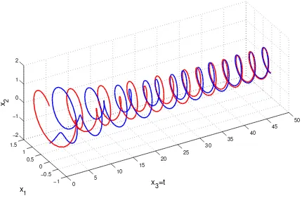
Figure 2.4. 3D phase portrait of a damped oscillator with excitation
The system equation is ¨x+ 0.16 ˙x+x= 1.2 cos 2.1t, the initial conditions are
We can also interpret such higher dimensional phase portraits, as a plot assem-bled from the different xi(t) plots. The similarity can be well observed in Figure
2.4. Looking at the phase portrait from “above” (parallel with the x2 axis), we
get x1(t), while from the “side” (parallel with the x1 axis) we see x2(t). We can
also notice how the trajectories approach a spiral with radius 1.2 after a tran-sient interval, which spiral has a projection of a periodic (in this case circular), closed trajectory on the x1, x2 plane. This spiral is in fact the 3D phase space
representation of the damped oscillators steady state solution.
2.3
Poincaré concept
Our motivation now is to find a tool to efficiently handle systems like the one in Figure 2.4. As mentioned above, after a transient, the system seems to approach a periodic state, oscillating around (x1, x2) = (0,0). This means, that if we look at
the phase space’s projection on thex1, x2 plane, the trajectories approach a circle,
centered at the origin, with radius equal to the excitation.
The idea is that this the convergence of the system could be defined by the convergence of a discrete time sequence, which we get by sampling the trajectories with a sampling rate f identical to the excitation frequency. Doing so, we get the sequencexn=Φ(tn), wheretn=nT, T=f−1 andn∈ {0,1,2. . .}. If the projection
ofΦ(x0, t) on thex1, x2 plane converges to a periodic curve (with the same period
as the excitation),xn will converge to a single point, as illustrated in Figure 2.5.
This method can be explained by placing equally distant (ts) planes along the
t axis, parallel to the x1, x2 plane. We will get xn by taking the intersection
points of Φ(tn) and the “sampling planes.” This is harder to imagine in higher
dimensions; for example in 4D, the subspace orthogonal to thetaxis will be three-dimensional. On the other hand, this approach will be closer to the one used later for autonomous systems.
Clearly, the location of the limit point depends on when we start the sampling, but as we will see later, the fact that it converges can be more important than the limit itself. Nevertheless, we can be sure that the limit point will be on the circle, or if the projections on the x1, x2 plane converge to a certain point, xn will do so
as well.
By converting the non-autonomous system to an autonomous one, Φ(x0, t0)
−1 −0.5 0 0.5 1 −1.5
−1 −0.5 0 0.5 1 1.5
x 1 x 2
−1 −0.5 0 0.5 1
−1.5 −1 −0.5 0 0.5 1 1.5
x 1 x 2
Figure 2.5. Projections of the trajectories in Figure2.4, with periodic samples
On the left figure, the sampling started attinit= 0, while on the right one, the
sampling started attinit=T /2. The time step in both cases correspond to the
frequency of the excitation,ω= 2.1, hence T =f−1
= 2π/ω.
sampling tinit. In other words, if a certain xi=Φ(ti) is given for a known system,
xi definesxi+1 uniquely, just like (x0, t0) defines the flow on which xn is located.
Formally, this leads to the recursive definition
xi+1=P(xi), xn=Pn(x0), (2.12)
where P :Rm→Rm is called the Poincaré-map. (For a general and more formal
definition of P, see [5].)
By introducing P, we have reduced the analysis of an (m+ 1)–dimensional phase space by 1 dimension, and also traced back the analysis of continuous curves to discrete time sequences. We have obviously used the fact, that the (m+ 1)– dimensional phase portrait has special features, inherited from 2.11. Now let us try to apply this method to autonomous systems, or systems without periodic excitation. The problem is that the sampling frequency is now undefined, or in other words, we do not know where to place the “sampling planes.”
Figure 2.6. Illustration of the Poincaré concept in non-autonomous (left) and
autonomous (right) systems[7]
As we do not have a “natural” sampling rate in many cases, we generalize the idea through its geometric interpretation: just as before, we are going to take samples as the intersection of a phase curve and a plane (or to be more general, a subspace 1 dimension lower than the original phase space). The difference is that we are going to use only one plane (from now on called the Poincaré plane), fixed in the phase space, and we will take into consideration only the intersection points which occur when the trajectory crosses the plane in one direction, neglecting the intersection points by the trajectory puncturing the plane on its way back.
−4 −2 0 2 4
−2.5 −2
−1.5 −1
−0.5 0
0.5 1 1.5 2 2.5 −4
−3 −2 −1 0 1 2 3 4
x
2
x
1 x 3
Figure 2.7. Trajectories of the system x(3)+ 4¨x+ 6 ˙x+ 4x= 0, with different placement of the Poincaré plane:
0 0.5 1 1.5 −0.5
−0.4 −0.3 −0.2 −0.1 0 0.1
x
2
x 3
Figure 2.8. Poincaré section of the system in Figure 2.7(x= 0) Note how the sequences approach (and in fact converge to) the origin.
Just as before, the Poincaré-map function defines the relation between two consecutive elements of the discrete time sequence. However, the way we choose the plane will affect our results heavily. As it can be seen in Figure 2.7, the plane will give us useful information about the system only if we place it at the correct location and with the correct orientation. The sequences represented by squares and diamonds, not only do not converge, but are also finite. In order to use this tool successfully, we will have to find the “interesting” parts of the phase space first, and then place the plane with the correct orientation. Now we have some tools to qualitatively analyze our systems. As it was implicitly indicated before, a system’s transient behavior is usually less of interest. However, the long term (or – if such exists – the final) state of the systems is very important. To investigate how the systems typically evolve, we can analyze trajectories and phase portraits, or use the Poincaré section.
2.4
Equilibrium points
a typical feature of 2D and 3D phase portraits, based on which we can classify systems.
Let us introduce what is called an equilibrium or fixed point. As the name indicates, if a system’s state reaches an equilibrium, the state will not change further. Formally, it can be expressed as x˙ = 0, which means that in order to find equilibria, we have to find the points x∗
k (where k denotes the index for the
equilibria points) which satisfy
0=f(x∗
k). (2.13)
When we find an equilibrium, the question of stability rises: if we apply some small perturbation to the system, will it go back to equilibrium or not, and how will it behave before it returns to its stable state or how will it diverge from an unstable equilibrium? In order to examine the system’s behavior after introducing some small perturbation ∆x, we have to expand the function around x∗
k, and
neglect the terms of order higher than one[8]:
f(x∗
k+ ∆x)≈f(x
∗
k) +Jk∆x, (2.14)
whereJkis the Jacobian matrix evaluated atx
∗
k, thereforeJkis time independent.
Then substituting back to 2.13 and 2.10 gives us a coupled system of n first order differential equations with constant coefficients, represented in matrix form as
d∆x
dt =Jk∆x. (2.15)
The solution of such system will be in the form of
∆x=eλte, (2.16)
which when substituted back to2.15 yields the eigenvalue equation of Jk:
Jke=λe. (2.17)
Thus, the characteristic equation of Jk will be
det(Jk−λI) = 0, (2.18)
where Iis the – m dimensional rectangular – identity matrix.
Without concerning the case of multiple and zero eigenvalues, 2.15 will have
by r ∈ {1,2, . . . , m}. Therefore we will have the eigenvalues λr, each uniquely
corresponding to an eigenvectorer, where{er}forms a basis. The general solution
will be
∆x=
m
X
r=1
eλrt
er, (2.19)
assuming that ∆x(t= 0) =
m
X
r=1
eλrt
. Knowing that we are considering only systems with real coefficients (Jk∈Rm×Rm), the eigenvalues will be either real, or they
will appear as complex conjugate pairs (so will the corresponding eigenvectors). The equilibrium point is called (linearly) stable, if all the real eigenvalues and the real parts of all complex conjugate pair roots are negative. In two dimensions (on the phase plane), both roots of the characteristic equation are either real or form complex conjugate pair. Regarding stability, we have 6 qualitatively different cases depending on the eigenvalues.
(a) 2D stable node (b) 2D stable focus
(c) 2D unstable node (d) 2D unstable focus
(e) 2D saddle point (f) 2D center
Table 2.1. Phase portraits of linearized 2D equilibria points [7]
These cases are (as illustrated in Table 2.1):
B) Focus, stable: complex conjugate eigenvalues with negative real part; the fixed point is stable, e.g. the damped harmonic oscillator in Figure 2.2. C) Node, unstable: both eigenvalues are positive real; the fixed point is unstable.
D) Focus, unstable: complex conjugate eigenvalues with positive real part; the the fixed point is unstable.
E) Saddle point: one eigenvalue is negative real, the other is positive real; the fixed point is unstable. The eigenvector corresponding to the negative eigen-value spans a one-dimensional subspace, which is a stable manifold.
F) Center, unstable: complex conjugate eigenvalues with zero real part; the fixed point is linearly unstable (but might be stable according to Lyapunov’s defini-tion – see later), e.g. the undamped harmonic oscillator or the mathematical pendulum in Figure 2.2.
(a) 3D (stable) node (b) 3D repeller (unstable node)
(c) 3D saddle point – Index 1 (d) 3D saddle point – Index 2
Table 2.2. Phase portraits of 3D equilibria with real eigenvalues [8]
In 3 dimensions, the case is more complicated. If all the eigenvalues are real, we have four different cases, illustrated in Table 2.2:
A) Node (stable): all three eigenvalues are negative; the fixed point is stable. B) Repeller (unstable node): all three eigenvalues are positive; the fixed point is
C) Saddle point – Index 1: two eigenvalues are negative, one is positive; the fixed point is unstable. The eigenvectors corresponding to the negative eigenvalues span a two-dimensional subspace, which is tangent to a stable manifold. D) Saddle point – Index 2: one eigenvalue is negative, two are positive; the fixed
point is unstable. The eigenvector corresponding to the negative eigenvalue spans a one-dimensional subspace, which is tangent to a stable manifold.
(a) 3D spiral node (b) 3D spiral repeller
(c) 3D spiral saddle point – Index 1 (d) 3D spiral saddle point – Index 2
Table 2.3. Phase portraits of 3D equilibria with one complex conjugate pair
eigenvalues [8]
In 3D only one complex conjugate pair can appear, and at least one of the roots is always real. In case of one complex conjugate pair and one real root, we also have four cases depending on the real parts of the complex conjugate pairs and the real root, illustrated in Table 2.3:
A) Spiral node: all the real parts are negative; the fixed point is stable. B) Spiral repeller: all the real parts are positive; the fixed point is unstable. C) Spiral saddle point – Index 1: the real part of the complex conjugate pair
D) Spiral saddle point – Index 2: the real part of the complex conjugate pair is positive, the real eigenvalue is negative; the fixed point is unstable. The eigen-vector corresponding to the negative real eigenvalue spans a one-dimensional subspace, which is tangent to a stable manifold.
Nodes and spiral nodes are called attractors, as solutions tend to converge to them. Linear stability can – and sometimes is – defined through this convergence, rather than giving the above definition through the spectrum of the Jacobian matrix (for which it is also called spectral stability).
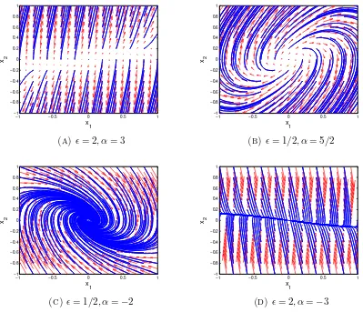
For a complex conjugate pair with zero real part, linearization predicts a similar circular pattern as in Figure 2.1f, yielding two qualitatively different cases, illus-trated in Figure 2.4. However, the effect of higher order terms neglected cannot be seen, therefore linearization in this case might easily give us a false picture of the system’s behavior at the fixed points.
(a) 3D center – Index 1 (b) 3D center – Index 2
Table 2.4. Phase portraits of 3D equilibria with one complex conjugate pair having zero real part
A) 3D center – Index 1: the real part of the complex conjugate pair is zero, the real eigenvalue is negative, the fixed point is linearly unstable (but might be stable according to Lyapunov’s definition – see later). The eigenvector cor-responding to the negative real eigenvalue spans a one-dimensional subspace, which is tangent to a stable manifold. The subspace spanned by the complex conjugate eigenvector pair is a result of linearization, and might give a false picture of the system’s behavior.
B) 3D center – Index 2: the real part of the complex conjugate pair is zero, the real eigenvalue is positive, the fixed point is unstable.
Figure2.7. On the other hand, we should not forget about the fact that these equi-librium phase portraits are the result of a rough approximation. The linearization obviously restricts the perturbation to small amplitudes. Moreover, neglecting nonlinear terms might (or might not) take its toll as the trajectories evolve fur-ther. In other words, the nonlinearity of the system can ruin our approximation regarding the system’s long-term behavior, even if the perturbation is relatively small. The linearized equation predicts exponential behavior around equilibria (therefore – surprisingly – also called exponential stability), which can suffice in case of attractors. However, for solutions diverging from the vicinity of (unstable) equilibria, linearization cannot tell anything about the fate of the system[9].
An interesting problem is when the first order term of the expansion yields zero. Consider the system ˙x= 1−e−x2
, where f(0) = 0, but f′
(0) = 0. It is impossible to determine by linearization ifxe= 0 is a 1D node (local minimum), 1D repeller
(local maximum) or a 1D saddle (inflection point). Similarly in higher dimensions, if Jk is singular (has zero eigenvalues) and ∆x∈ker(Jk) a different approach is
needed.
Nevertheless, if an attractor is found, we can be sure that there exists a do-main in the phase space, from which the solutions converge to the attractor. The manifold (i.e. set of points in phase space) from which the solutions converge to the attractor is called the basin of attraction. If the system parameters are not changed (thus no excitation is applied either), solutions will not enter or leave the basin of attraction. We could say, that trajectories “born” in a basin (meaning their initial state is in the basin) never leave and external trajectories cannot cross the boundary of the basin either, making it easier to find the basin of attraction (e.g. with numerical methods) after the attractor itself is found.
The subspaces spanned by the eigenvectors of Jk correspond to and are
tan-gent to manifolds of the fixed point x∗
k. To each stable subspace belongs a stable
manifold, from which the trajectories approach the fixed point. Likewise, to each unstable subspace belongs an unstable manifold, from which the trajectories di-verge from the fixed point. The eigenvectors belonging to zero eigenvalues and to complex conjugate pairs with zero real parts also span a subspace, which is tangent to a so called center manifold. This center manifold usually shows inter-esting phenomena as linearization does not predict its behavior, not even on short term[10].
Figure 2.9. Basins of attraction [8]
dictates that we could consider an equilibrium stable if for a finite perturbation, it does not leave a finite region around the equlibrium. Formally, if for everyǫ∈R+
exists δ(ǫ)∈R+ such that if ||x(0)−x∗
k||< δ, then ||x(t)−x
∗
k||< ǫ, for ∀t∈R+.
This is called Lyapunov stability[11] and it is often used in control theory.
2.5
Closed trajectories
So far we have seen three typical type of trajectories in planar systems. Open trajectories start at non-equilibrium points and can go on forever diverging to infinity or converging to a stable equilibrium. Fixed points themselves are degen-erate solutions, where the trajectories are single points. The third case is when the state of the system changes periodically, resulting in closed curves on the phase portrait as seen on Figure 2.1f and the 2D subspaces on Figure2.4.
The closed curves described before were the results of linearization around an equilibrium point which was linearly unstable (but could be stable according to Lyapunov’s definition). However. we did not question the stability of a periodical solution so far. For the above mentioned closed curves, a small perturbation would force the solution to a different closed curve, where it would start its infinite period again. As it can be seen on Figure2.10, perturbing the periodic solution too much can force the system to a different kind of trajectory.
−6 −4 −2 0 2 4 6 −2
−1.5 −1 −0.5 0 0.5 1 1.5 2
φ
ω
Figure 2.10. Phase portrait of the (rigid) mathematical pendulum
Note the centers at (φ, ω) = (2kπ,0) corresponding to the Lyapunov stable
equi-libria and the saddle points at (φ, ω) = ((2k+ 1)π,0) corresponding to the
un-stable equilibria (k∈Z). The curves (red and green) connecting the two saddle
points are heteroclinic orbits. Together they form a closed loop.
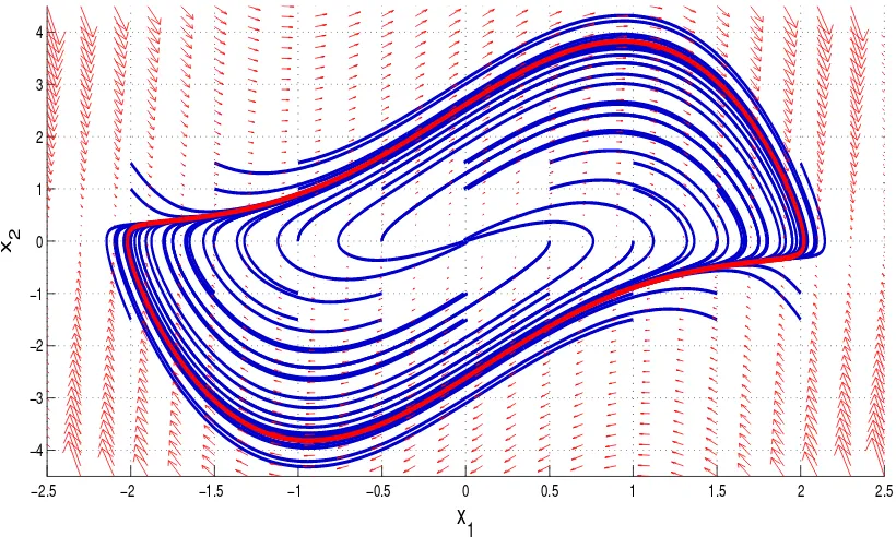
systems was described and can be seen on Figure 2.5, where the excitation forces the system to a periodic orbit. This new kind of trajectory is called a (stable) limit cycle, as it is a limit set of another trajectories. The exact difference between closed curves around a center and limit cycles is that limit cycles are isolated, meaning there are no other periodic solutions nearby (other limit cycles can exist, but a finite distance has to be between two of them).
Stable limit cycles are relaxation oscillations, meaning that the system oscillates without excitation. Such self-sustained periodic motion is unique to nonlinear systems (the closed orbits of linear systems are never isolated)[12] and are always a subject of interest when one is found. Numerous examples of limit cycles can be found in biological systems, including the beating of the heart, breathing and rhythms in body temperature.
The closed curves (including limit cycles) seen so far had finite periods. Another kind of closed trajectories can be created by connecting what is called heteroclinic orbits. Heteroclinic orbits are curves in the phase space which connect two different equilibrium points. Because x˙ =v= 0 at fixed points, the velocity v decreases along a heteroclinic orbit, thus the trajectory only reaches the equilibrium when
−1 −0.8 −0.6 −0.4 −0.2 0 0.2 0.4 0.6 0.8 1 −1
−0.8 −0.6 −0.4 −0.2 0 0.2 0.4 0.6 0.8 1
x
y
Figure 2.11. Example of a heteroclinic connection[5]
The system is defined as ˙x=y+x2−x
4(y−1 + 2x2),y˙=−2x(1 +y).
Note the saddle points at (−1,−1) and (−1,1) connected by the two heteroclinic
curves. Solutions starting near the unstable node at (0,0) converge to the closed
loop, but solutions starting outside the loop diverge over time. Thus this orbit is semi-stable.
In a similar manner, a curve can be closed by starting at a saddle point and after forming a loop, ending up in the same point (Figure 2.12). In this case the stable and unstable manifolds of the saddle point overlap. This curve in the phase space is called a homoclinic orbit[14]. According to [5], only one heteroclinic orbit may exist between two fixed points (in one direction), but there are no restrictions regarding the number of homoclinic orbits associated with a saddle point. There might even be an infinite number of homoclinic orbits connected to a single fixed point.
While fixed points were easy to find by (either analytically or numerically) solving 2.13, there is very little known about finding limit cycles. Numerical methods exist, but in order to succeed we need to know where to look. However for planar systems, the Poincaré-Bendixson theorem[5, 12] states that if a trajectory is confined to a closed and bounded domain on the phase plane containing finitely many fixed point, the trajectory converges
a) to a fixed point. b) to a limit cycle.
−1 −0.8 −0.6 −0.4 −0.2 0 0.2 0.4 0.6 0.8 1 −1
−0.5 0 0.5 1
x
y
Figure 2.12. Example of homoclinic orbits[5]
The system is defined as ˙x=y,y˙=−ηxE(x, y)2−U′
(x), whereE(x, y)=y22+U(x),
U(x) =x4−x2 and η= 0.1.
Therefore the existence of a limit cycle in 2D can be proven by finding a bounded finite region which does not contain fixed points and proving that there exist one trajectory which does not leave this region for t→ ∞. Unfortunately this theorem does not hold for higher dimensional systems. Periodic solutions in the three-dimensional phase space can be found using the Poincaré concept (Figure
2.5). However, not only do these solutions become more difficult to find in higher dimensions, new kinds of trajectories appear along the ones described above.
−1.5 −1 −0.5 0 0.5 1 1.5
−1.5 −1 −0.5 0 0.5 1 1.5
x
y
Figure 2.13. Phase portrait of the system given in the following polar form: ˙
r=r(1−r2),φ˙= 1(r>0)
The limit cycle at r=p
2.6
Quasi-periodic oscillations and
frequency-locked loops
Using the Poincaré concept on a 2D limit cycles such as on Figure 2.13 will yield a sequence of converging points. In this case the point of convergence on the Poincaré plane corresponds to an attractor (a stable limit cycle) on the phase plane. A 2D stable focus will also appear as a limit point on the Poincaré plane, similarly to what is described on Figure 2.8. Both cases lead to a mapping P for which the point of convergencex∗
is an invariant point meaning that P(x∗
) =x∗
. For 2D continuous systems this is necessary and sufficient condition for finding fixed points or limit cycles. If limn→∞Pn(x0) = x
∗
, we can say that it is an attractor (stable limit cycle or stable focus).
Similarly in higher dimensions if such point of convergence is found, it indicates an attractor. On the other hand, the reverse statement is not true, an attractor can appear differently on the Poincaré plane. A frequency-locked loop is a closed trajectory composed of multiple periodic motions with different angular frequen-cies, which frequencies are commensurate (i.e. their ratio is rational)[8].
Figure 2.14. Frequency-locked loop on the surface of a torus. The frequencies
areωR= 3, ωr= 1 with the corresponding amplitudes (major and minor radii of
the torus)R= 5, r= 1
Such state is easy to demonstrate as a trajectory on the surface of a torus, as it is shown on Figure 2.14. For such, there is no point of convergence on the Poincaré plane and the section points x∗
1,x
∗
2,x
∗
3 of the loop are not invariant
points of P. On the other hand, the loop appears as a periodic sequence as
P3(x∗
3) =P2(x
∗
1) =P(x
∗
2) =x
∗
Figure 2.15. Trajectories converging to a frequency-locked loop attractor
described on Figure 2.14(for larger see FigureC.1)
−6 −5.5 −5 −4.5 −4 −1 −0.8 −0.6 −0.4 −0.2 0 0.2 0.4 0.6 0.8 1
x2
x3
(a)Poincaré section of Figure2.14
−6 −5.5 −5 −4.5 −4 −1 −0.8 −0.6 −0.4 −0.2 0 0.2 0.4 0.6 0.8 1
x2
x3
(b)Poincaré section of Figure2.15
Figure 2.16. Poincaré sections of frequency-locked loops
to this periodic sequence, and the section points approach x∗
1,x
∗
2,x
∗
3, as they do
on Figure 2.16b.
When the frequencies are not commensurate, meaning their ratio is is not ratio-nal the orbit on the surface of the torus does not close. This is called quasi-periodic oscillation as the components are periodic but the trajectory is not. Over time, the trajectory on the torus will form a dense pattern, thus the trajectory will get arbitrarily close to any point on the torus. This is phenomenon is similar to what Lissajous-curves exhibit in 2D with non-commensurate x and y frequencies.
(a) Quasi-periodic motion in the phase space
−6 −5.5 −5 −4.5 −4 −1 −0.8 −0.6 −0.4 −0.2 0 0.2 0.4 0.6 0.8 1
x2
x3
(b) Poincaré section of
Figure2.17a
Figure 2.17. Quasi-periodic oscillation on a torus. The frequencies areωR=
2, ωr= 3π with the corresponding amplitudes (major and minor radii of the
torus)R= 5, r= 1
Poincaré concept be utilized, that it decreases the dimension of the system by one and traces back the examination of a continuous system to a discrete mapping. Quasi-periodic and frequency-locked motions can appear in higher dimensional systems as well. In this case the motion consists of m frequencies and it can be imagined as trajectories on the surface of an m-dimensional torus embedded in the m+ 1-dimensional phase space.
The equilibria points, the limit cycles, frequency-locked loops and quasi-periodic oscillations are called regular attractors (if they are stable)[8]. Their common fea-ture is predictability: small changes in the initial conditions will stay small as the trajectories evolve and approach the attractor over time. The lack of this predictability is one of the most important feature of the systems that will be discussed in the following.
2.7
Chaotic state
In his paper with which he won the prize of Oscar II, Henri Poincaré made a mistake[4]. Later he realized his mistake and corrected it, which lead to the first encounter of which was later called chaotic state. He considered equations in the form
˙
x=f(x) +ǫg(x, t), (2.20) where ǫ is small andg(x, t) is periodic in t [15].
(a) Homoclinic intersection
(b) Homoclinic tangle
Figure 2.18. The forming of a homoclinic tangle (source: [15])
lied in his assumption that perturbation could break this surface, which lead him to false conclusions regarding the stability of the solution[15]. He later realized that the perturbation usually breaks the homoclinic orbits into two intersecting curves, of which he showed that they must intersect each other infinitely many times[16] without ever reaching the equilbrium point. This would create a complicated web of solutions, where stability could never be reached[15].
The chaos as defined today is a relatively new concept. Although related phe-nomena were encountered by a number scientists in the first half of the 20th century, the chaotic state of systems was first recognized by Edward Lorenz in the 1960s. Even though a formal definition of chaos does not exist, there are conditions which have to be met and common features of chaotic systems are known[8].
– The system is deterministic, meaning that the equation describing it is known and does not contain random terms. Chaotic systems show random-like behavior but it is mathematically deterministic.
– Nonlinearity: chaotic state does not appear in finite dimensional linear systems (but it can in infinite dimensional linear systems).
– Chaos can only appear in continuous systems of a dimension at least 3, given no excitation. For non-autonomous systems this limit is 2 (as these systems can be transformed into 3 dimensional autonomous system). However, chaotic states may be attained in discrete systems of dimension as low as 1.
changes or the lack of precision of setting the initial conditions) will make a false impression of randomness in the system. This, on the other hand, is not to be confused with the real randomness of quantum-level systems or the concept of randomness in statistics. For such reasons, it is sometimes referred to as deterministic chaos.
– Nearby trajectories diverge with an exponential rate (see Lyapunov exponent). – The trajectories are bounded and non-periodic. Quasi-periodic oscillations de-scribed in Section2.6are not chaotic, as they solutions starting near each other stay close as they evolve.
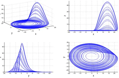
– Trajectories are attracted to a so called strange attractor. This attractor has a zero measure and a sophisticated fractal structure. An example can be seen on Figure2.19.
−20 −10
0 10
20
−20 0 200 10 20 30 40
x y
z
−200 −15 −10 −5 0 5 10 15 20
10 20 30 40
x
z
−20 −15 −10 −5 0 5 10 15 20 0 10 20 30 40
y
z
−20 −15 −10 −5 0 5 10 15 20
−20 −15 −10 −5 0 5 10 15 20
x
y
Figure 2.19. Example of a strange attractor
The Rössler system is defined as ˙x=−y−z, ˙y=x+ay, ˙z=b+z(x−c). The
strange attractor is plotted with the parameters a=b= 0.1, c= 14. Because
of the complicated fractal structure of the attractor and the non-periodicity of the chaotic state, strange attractors can be visualized by plotting only one
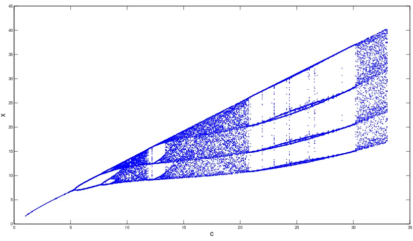
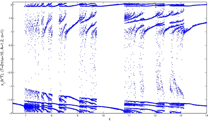
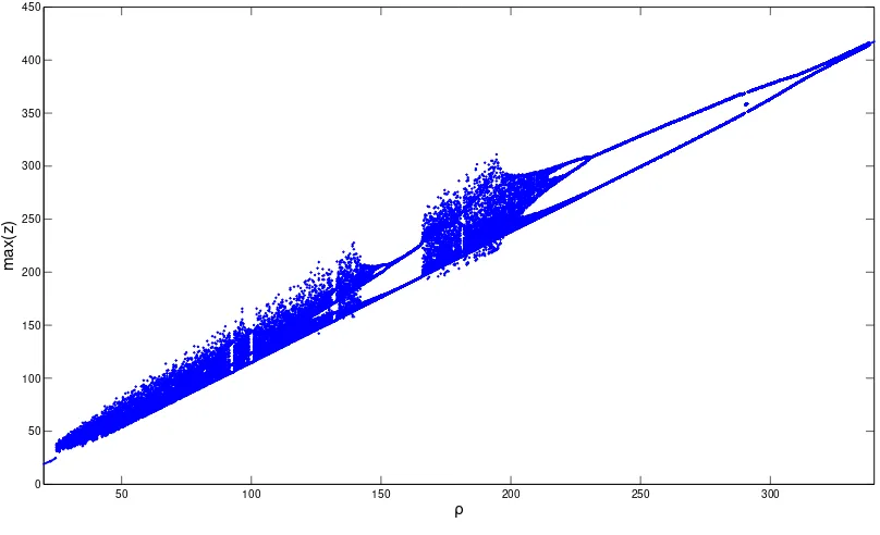
A given system may have a chaotic attractor at certain parameter values but may have a regular attractor for others. Thus it makes sense to examine how the changes in one of the system parameters change the stability of the system. To do so, first we start trajectories from somewhere in the basin of attraction, with different system parameters (typically changing only one parameter, while keeping others the same). The exact initial values are not important, as long as they are inside the basins of attraction of the chaotic and regular attractors. After some transient we take the Poincaré section of the system somewhere in the domain of interest. The exact position of the plane is again not important, as long as it crosses the attractors.
On the Poincaré plane we will have limit points corresponding to the regu-lar periodic attractors and section points where the chaotic trajectories cross the plane, as they do not show any periodicity, not even after the transient. The last step is to take on of the coordinates of the section point and plot it against the the changing system parameter. This diagram is called a bifurcation diagram of a system. This diagram shows the long term behavior of the system as a func-tion of a chosen systems parameter (a coefficient in f(x)) called the bifurcation parameter.
If we are not interested in the quantitative behavior of the Poincaré map func-tion, there is another way to create bifurcation diagrams. Finding the local max-imum (or minmax-imum) values of a state variable xi(t) in time and plotting them
against the bifurcation parameter is usually easier to implement in code or on measured data. However, this might conceal frequency-locked scenarios, where the peaks are at similar value during the multiple periods. E.g. on Figure 2.15, where this algorithm would indicate the same peaks in the vertical (z) direction. Nevertheless, it works fine for most of the systems.
0 5 10 15 20 25 30 35 0
5 10 15 20 25 30 35 40 45
c
x
Figure 2.20. Bifurcation diagram of the Rössler system defined in Figure2.19
The system paramteres a and b are kept at a constant value of 0.1, while c is
changing. (For larger see FigureC.3)
In fact, the period doubling does not stop at period 8, but happens infinitely many times before the systems turns to a chaotic state. The point where the pe-riod doubling stops and chaos emerges is called Feigenbaum point after American mathematical physicist Mitchell Feigenbaum. His work led to the discovery of two constants also named after him[8]. The first Feigenbaum constant is defined as
δ= lim
k→∞
µk−1−µk−2
µk−µk−1
≈4.669, (2.21)
where µk is the value of the bifurcation parameter µ at the kth bifurcation. The
second Feigenbaum constant is defined as
α= lim
k→∞
(∆x)k
(∆x)k+1
≈2.503, (2.22)
where (∆x)k is the distance between the two ends of a bifurcation fork in x
di-rection at the kth bifurcation. It turns out that these constants are universal to any system’s period-doubling bifurcation, thus these constants are fundamental in chaos theory[8].
−20 −15 −10 −5 0 5 10 15 20 −20 −15 −10 −5 0 5 10 15 x y
(a) c= 4, period 1
−20 −15 −10 −5 0 5 10 15 20 −20 −15 −10 −5 0 5 10 15 x y
(b) c= 6.5, period 2
−20 −15 −10 −5 0 5 10 15 20 −20 −15 −10 −5 0 5 10 15 x y
(c) c= 8.5 period 4
−20 −15 −10 −5 0 5 10 15 20 −20 −15 −10 −5 0 5 10 15 20 x y
(d) c= 8.7 period 8
−20 −15 −10 −5 0 5 10 15 20 −20 −15 −10 −5 0 5 10 15 20 x y
(e) c
![Figure 2.3. Example of a phase portrait with the vector field[The system plotted is defined by ˙6]x1 = −x1 −2x2x21 +x2,x˙2 = −x1 −x2](https://thumb-ap.123doks.com/thumbv2/123dok/1394814.1517454/21.596.102.519.465.713/figure-example-phase-portrait-vector-eld-plotted-dened.webp)