SciPy and NumPy Free ebook download

(1)

(2)

SciPy and NumPy

Eli Bressert

(3)

SciPy and NumPy by Eli Bressert

Published by O’Reilly Media, Inc., 1005 Gravenstein Highway North, Sebastopol, CA 95472.

O’Reilly books may be purchased for educational, business, or sales promotional use. Online editions are also available for most titles (http://my.safaribooksonline.com). For more information, contact our corporate/institutional sales department: (800) 998-9938 orcorporate@oreilly.com.

Interior Designer: David Futato Project Manager: Paul C. Anagnostopoulos Cover Designer: Randy Comer Copyeditor: MaryEllen N. Oliver Editors: Rachel Roumeliotis, Proofreader: Richard Camp

Meghan Blanchette Illustrators: Eli Bressert, Laurel Muller Production Editor: Holly Bauer

November 2012: First edition

Revision History for the First Edition:

2012-10-31 First release

Seehttp://oreilly.com/catalog/errata.csp?isbn=0636920020219for release details.

Nutshell Handbook, the Nutshell Handbook logo, and the O’Reilly logo are registered trademarks of O’Reilly Media, Inc.SciPy and NumPy, the image of a three-spined stickleback, and related trade dress are trademarks of O’Reilly Media, Inc.

Many of the designations used by manufacturers and sellers to distinguish their products are claimed as trademarks. Where those designations appear in this book, and O’Reilly Media, Inc., was aware of a trademark claim, the designations have been printed in caps or initial caps.

While every precaution has been taken in the preparation of this book, the publisher and authors assume no responsibility for errors or omissions, or for damages resulting from the use of the information contained herein.

(4)

4. SciKit: Taking SciPy One Step Further . . . 43

4.1 Scikit-Image 43

4.2 Scikit-Learn 48

5. Conclusion . . . 55

5.1 Summary 55

5.2 What’s Next? 55

(5)

(6)

Preface

Python, a high-level language with easy-to-read syntax, is highly ﬂexible, which makes it an ideal language to learn and use. For science and R&D, a few extra packages are used to streamline the development process and obtain goals with the fewest steps possible. Among the best of these are SciPy and NumPy. This book gives a brief overview of different tools in these two scientiﬁc packages, in order to jump start their use in the reader’s own research projects.

NumPy and SciPy are the bread-and-butter Python extensions for numerical arrays and advanced data analysis. Hence, knowing what tools they contain and how to use them will make any programmer’s life more enjoyable. This book will cover their uses, ranging from simple array creation to machine learning.

Audience

Anyone with basic (and upward) knowledge of Python is the targeted audience for this book. Although the tools in SciPy and NumPy are relatively advanced, using them is simple and should keep even a novice Python programmer happy.

Contents of this Book

This book covers the basics of SciPy and NumPy with some additional material. The ﬁrst chapter describes what the SciPy and NumPy packages are, and how to access and install them on your computer. Chapter 2 goes over the basics of NumPy, starting with array creation. Chapter 3, which comprises the bulk of the book, covers a small sample of the voluminous SciPy toolbox. This chapter includes discussion and examples on integration, optimization, interpolation, and more. Chapter 4 discusses two well-known scikit packages: scikit-image and scikit-learn. These provide much more advanced material that can be immediately applied to real-world problems. In Chapter 5, the conclusion, we discuss what to do next for even more advanced material.

(7)

Conventions Used in This Book

The following typographical conventions are used in this book:

Plain text

Indicates menu titles, menu options, menu buttons, and keyboard accelerators (such as Alt and Ctrl).

Italic

Indicates new terms, URLs, email addresses, ﬁlenames, ﬁle extensions, pathnames, directories, and Unix utilities.

Constant width

Indicates commands, options, switches, variables, attributes, keys, functions, types, classes, namespaces, methods, modules, properties, parameters, values, objects, events, event handlers, XML tags, HTML tags, macros, the contents of ﬁles, or the output from commands.

This icon signiﬁes a tip, suggestion, or general note.

This icon indicates a warning or caution.

Using Code Examples

This book is here to help you get your job done. In general, you may use the code in this book in your programs and documentation. You do not need to contact us for permission unless you’re reproducing a signiﬁcant portion of the code. For example, writing a program that uses several chunks of code from this book does not require permission. Selling or distributing a CD-ROM of examples from O’Reilly books does require permission. Answering a question by citing this book and quoting example code does not require permission. Incorporating a signiﬁcant amount of example code from this book into your product’s documentation does require permission.

We appreciate, but do not require, attribution. An attribution usually includes the title, author, publisher, and ISBN. For example: “SciPy and NumPyby Eli Bressert (O’Reilly). Copyright 2013 Eli Bressert, 978-1-449-30546-8.”

If you feel your use of code examples falls outside fair use or the permission given above, feel free to contact us atpermissions@oreilly.com.

We’d Like to Hear from You

(8)

O’Reilly Media, Inc.

1005 Gravenstein Highway North Sebastopol, CA 95472

(800) 998-9938 (in the United States or Canada) (707) 829-0515 (international or local)

(707) 829-0104 (fax)

We have a web page for this book, where we list errata, examples, links to the code and data sets used, and any additional information. You can access this page at:

http://oreil.ly/SciPy_NumPy

To comment or ask technical questions about this book, send email to:

bookquestions@oreilly.com

For more information about our books, courses, conferences, and news, see our website athttp://www.oreilly.com.

Find us on Facebook:http://facebook.com/oreilly

Follow us on Twitter:http://twitter.com/oreillymedia

Watch us on YouTube:http://www.youtube.com/oreillymedia

Safari® Books Online

Safari Books Online (www.safaribooksonline.com) is an on-demand digital library that delivers expert content in both book and video form from the world’s leading authors in technology and business.

Technology professionals, software developers, web designers, and business and cre-ative professionals use Safari Books Online as their primary resource for research, problem solving, learning, and certiﬁcation training.

Safari Books Online offers a range of product mixes and pricing programs for organi-zations, government agencies, and individuals. Subscribers have access to thousands of books, training videos, and prepublication manuscripts in one fully searchable data-base from publishers like O’Reilly Media, Prentice Hall Professional, Addison-Wesley Professional, Microsoft Press, Sams, Que, Peachpit Press, Focal Press, Cisco Press, John Wiley & Sons, Syngress, Morgan Kaufmann, IBM Redbooks, Packt, Adobe Press, FT Press, Apress, Manning, New Riders, McGraw-Hill, Jones & Bartlett, Course Technol-ogy, and dozens more. For more information about Safari Books Online, please visit us online.

Acknowledgments

I would like to thank Meghan Blanchette and Julie Steele, my current and previous editors, for their patience, help, and expertise. This book wouldn’t have materialized without their assistance. The tips, warnings, and package tools discussed in the book

(9)

(10)

CHAPTER 1

Introduction

Python is a powerful programming language when considering portability, ﬂexibility, syntax, style, and extendability. The language was written by Guido van Rossum with clean syntax built in. To deﬁne a function or initiate a loop, indentation is used instead of brackets. The result is profound: a Python programmer can look at any given uncommented Python code and quickly understand its inner workings and purpose.

Compiled languages like Fortran and C are natively much faster than Python, but not necessarily so when Python is bound to them. Using packages like Cythonenables Python to interface with C code and pass information from the C program to Python and vice versa through memory. This allows Python to be on par with the faster languages when necessary and to use legacy code (e.g.,FFTW). The combination of Python with fast computation has attracted scientists and others in large numbers. Two packages in particular are the powerhouses of scientiﬁc Python: NumPy and SciPy. Additionally, these two packages makes integrating legacy code easy.

1.1 Why SciPy and NumPy?

The basic operations used in scientific programming include arrays, matrices, integra-tion, differential equation solvers, statistics, and much more. Python, by default, does not have any of these functionalities built in, except for some basic mathematical op-erations that can only deal with a variable and not an array or matrix. NumPy and SciPy are two powerful Python packages, however, that enable the language to be used efficiently for scientific purposes.

NumPy specializes in numerical processing through multi-dimensional ndarrays, where the arrays allow element-by-element operations, a.k.a. broadcasting. If needed, linear algebra formalism can be used without modifying the NumPy arrays before-hand. Moreover, the arrays can be modiﬁed in size dynamically. This takes out the worries that usually mire quick programming in other languages. Rather than creating a new array when you want to get rid of certain elements, you can apply a mask to it.

(11)

SciPy is built on the NumPy array framework and takes scientiﬁc programming to a whole new level by supplying advanced mathematical functions like integration, ordinary differential equation solvers, special functions, optimizations, and more. To list all the functions by name in SciPy would take several pages at minimum. When looking at the plethora of SciPy tools, it can sometimes be daunting even to decide which functions are best to use. That is why this book has been written. We will run through the primary and most often used tools, which will enable the reader to get results quickly and to explore the NumPy and SciPy packages with enough working knowledge to decide what is needed for problems that go beyond this book.

1.2 Getting NumPy and SciPy

Now you’re probably sold and asking, “Great, where can I get and install these pack-ages?” There are multiple ways to do this, and we will ﬁrst go over the easiest ways for OS X, Linux, and Windows.

There are two well-known, comprehensive, precompiled Python packages that include NumPy and SciPy, and that work on all three platforms: the Enthought Python Dis-tribution (EPD) and ActivePython (AP). If you would like the free versions of the two packages, you should download EPD Free1_{or AP Community Edition.}2_{If you need}

support, then you can always opt for the more comprehensive packages from the two sources.

Optionally, if you are a MacPorts3user, you can install NumPy and SciPy through the package manager. Use the MacPorts command as given below to install the Python packages. Note that installing SciPy and NumPy with MacPorts will take time, espe-cially with the SciPy package, so it’s a good idea to initiate the installation procedure and go grab a cup of tea.

sudo port install py27-numpy py27-scipy py27-ipython

MacPorts supports several versions of Python (e.g., 2.6 and 2.7). So, althoughpy27is listed above, if you would like to use Python 2.6 instead with SciPy and NumPy then you would simply replacepy27withpy26.

If you’re using a Debian-based Linux distro like Ubuntu or Linux Mint, then use apt-get to install the packages.

sudo apt-get install python-numpy python-scipy

With an RPM-based system like Fedora or OpenSUSE, you can install the Python packages using yum.

sudo yum install numpy scipy

(12)

Building and installing NumPy and SciPy on Windows systems is more complicated than on the Unix-based systems, as code compilation is tricky. Fortunately, there is an excellent compiled binary installation program called python(x,y)4that has both NumPy and SciPy included and is Windows speciﬁc.

For those who prefer building NumPy and SciPy from source, visitwww.scipy.org/ Downloadto download from either the stable or bleeding-edge repositories. Or clone the code repositories from scipy.github.com and numpy.github.com. Unless you’re a pro at building packages from source code and relish the challenge, though, I would recommend sticking with the precompiled package options as listed above.

1.3 Working with SciPy and NumPy

You can work with Python programs in two different ways: interactively or through scripts. Some programmers swear that it is best to script all your code, so you don’t have to redo tedious tasks again when needed. Others say that interactive programming is the way to go, as you can explore the functionalities inside out. I would vouch for both, personally. If you have a terminal with the Python environment open and a text editor to write your script, you get the best of both worlds.

For the interactive component, Ihighlyrecommend using IPython.5It takes the best of the bash environment (e.g., using the tab button to complete a command and changing directories) and combines it with the Python environment. It does far more than this, but for the purpose of the examples in this book it should be enough to get it up and running.

Bugs in programs are a fact of life and there’s no way around them. Being able to ﬁnd bugs and ﬁx them quickly and easily is a big part of successful programming. IPython contains a feature where you can debug a buggy Python script by typingdebugafter running it. Seehttp:/ /ipython.org/ipython-doc/stable/interactive/tutorial.htmlfor details under the debugging section.

4_{http://code.google.com/p/pythonxy/} 5_{http://ipython.org/}

(13)

(14)

CHAPTER 2

NumPy

2.1 NumPy Arrays

NumPy is the fundamental Python package for scientiﬁc computing. It adds the capa-bilities ofN-dimensional arrays, element-by-element operations (broadcasting), core mathematical operations like linear algebra, and the ability to wrap C/C++/Fortran code. We will cover most of these aspects in this chapter by ﬁrst covering what NumPy arrays are, and their advantages versus Python lists and dictionaries.

Python stores data in several different ways, but the most popular methods arelists

anddictionaries. The Pythonlistobject can store nearly any type of Python object as an element. But operating on the elements in a list can only be done through iterative loops, which is computationally inefﬁcient in Python. The NumPy package enables users to overcome the shortcomings of the Python lists by providing a data storage object calledndarray.

Thendarrayis similar to lists, but rather than being highly flexible by storing different types of objects in one list, only the same type of element can be stored in each column. For example, with a Python list, you could make the first element a list and the second another list or dictionary. With NumPy arrays, you can only store the same type of element, e.g., all elements must be floats, integers, or strings. Despite this limitation, ndarraywins hands down when it comes to operation times, as the operations are sped up significantly. Using the%timeitmagic command in IPython, we compare the power of NumPyndarrayversus Python lists in terms of speed.

import numpy as np

# Create an array with 10^7 elements. arr = np.arange(1e7)

# Converting ndarray to list larr = arr.tolist()

# Lists cannot by default broadcast, # so a function is coded to emulate # what an ndarray can do.

(15)

def list_times(alist, scalar): for i, val in enumerate(alist):

alist[i] = val * scalar return alist

# Using IPython's magic timeit command timeit arr * 1.1

>>> 1 loops, best of 3: 76.9 ms per loop

timeit list_times(larr, 1.1)

>>> 1 loops, best of 3: 2.03 s per loop

Thendarrayoperation is ∼25 faster than the Python loop in this example. Are you convinced that the NumPyndarrayis the way to go? From this point on, we will be working with the array objects instead of lists when possible.

Should we need linear algebra operations, we can use thematrixobject, which does not use the default broadcast operation fromndarray. For example, when you multiply two equally sizedndarrays, which we will denote asAandB, theni,jelement ofAis only

multiplied by theni,j element ofB. When multiplying twomatrixobjects, the usual

matrix multiplication operation is executed.

Unlike thendarrayobjects,matrixobjects can and only will be two dimensional. This means that trying to construct a third or higher dimension is not possible. Here’s an example.

# Creating a 3D numpy array arr = np.zeros((3,3,3))

# Trying to convert array to a matrix, which will not work mat = np.matrix(arr)

# "ValueError: shape too large to be a matrix."

If you are working with matrices, keep this in mind.

2.1.1 Array Creation and Data Typing

There are many ways to create an array in NumPy, and here we will discuss the ones that are most useful.

# First we create a list and then # wrap it with the np.array() function. alist = [1, 2, 3]

arr = np.array(alist)

# Creating an array of zeros with five elements arr = np.zeros(5)

(16)

# Or 10 to 100? arr = np.arange(10,100)

# If you want 100 steps from 0 to 1... arr = np.linspace(0, 1, 100)

# Or if you want to generate an array from 1 to 10 # in log10 space in 100 steps...

arr = np.logspace(0, 1, 100, base=10.0)

# Creating a 5x5 array of zeros (an image) image = np.zeros((5,5))

# Creating a 5x5x5 cube of 1's

# The astype() method sets the array with integer elements. cube = np.zeros((5,5,5)).astype(int) + 1

# Or even simpler with 16-bit floating-point precision... cube = np.ones((5, 5, 5)).astype(np.float16)

When generating arrays, NumPy will default to the bit depth of the Python environ-ment. If you are working with 64-bit Python, then your elements in the arrays will default to 64-bit precision. This precision takes a fair chunk memory and is not al-ways necessary. You can specify the bit depth when creating arrays by setting the data type parameter (dtype) toint,numpy.float16,numpy.float32, ornumpy.float64. Here’s an example how to do it.

# Array of zero integers arr = np.zeros(2, dtype=int)

# Array of zero floats

arr = np.zeros(2, dtype=np.float32)

Now that we have created arrays, we can reshape them in many other ways. If we have a 25-element array, we can make it a 5×5 array, or we could make a 3-dimensional array from a ﬂat array.

# Creating an array with elements from 0 to 999 arr1d = np.arange(1000)

# Now reshaping the array to a 10x10x10 3D array arr3d = arr1d.reshape((10,10,10))

# The reshape command can alternatively be called this way arr3d = np.reshape(arr1s, (10, 10, 10))

# Inversely, we can flatten arrays arr4d = np.zeros((10, 10, 10, 10)) arr1d = arr4d.ravel()

print arr1d.shape (1000,)

The possibilities for restructuring the arrays are large and, most importantly, easy.

(17)

Keep in mind that the restructured arrays above are just different views of the same data in memory. This means that if you modify one of the arrays, it will modify the others. For example, if you set the ﬁrst element ofarr1dfrom the example above to1, then the ﬁrst element ofarr3dwill also become1. If you don’t want this to happen, then use thenumpy.copy function to separate the arrays memory-wise.

2.1.2 Record Arrays

Arrays are generally collections of integers or floats, but sometimes it is useful to store more complex data structures where columns are composed of different data types. In research journal publications, tables are commonly structured so that some col-umns may have string characters for identification and floats for numerical quantities. Being able to store this type of information is very beneficial. In NumPy there is the numpy.recarray. Constructing arecarrayfor the first time can be a bit confusing, so we will go over the basics below. The first example comes from the NumPy documentation on record arrays.

# Creating an array of zeros and defining column types recarr = np.zeros((2,), dtype=('i4,f4,a10'))

toadd = [(1,2.,'Hello'),(2,3.,"World")] recarr[:] = toadd

The dtype optional argument is defining the types designated for the first to third columns, wherei4 corresponds to a 32-bit integer, f4 corresponds to a 32-bit float, and a10corresponds to a string 10 characters long. Details on how to define more types can be found in the NumPy documentation.1This example illustrates what the recarraylooks like, but it is hard to see how we could populate such an array easily. Thankfully, in Python there is a global function calledzipthat will create a list of tuples like we see above for thetoaddobject. So we show how to usezipto populate the same recarray.

# Creating an array of zeros and defining column types recarr = np.zeros((2,), dtype=('i4,f4,a10'))

# Now creating the columns we want to put # in the recarray

col1 = np.arange(2) + 1

col2 = np.arange(2, dtype=np.float32) col3 = ['Hello', 'World']

# Here we create a list of tuples that is # identical to the previous toadd list. toadd = zip(col1, col2, col3)

# Assigning values to recarr recarr[:] = toadd

(18)

# Assigning names to each column, which

# are now by default called 'f0', 'f1', and 'f2'.

recarr.dtype.names = ('Integers' , 'Floats', 'Strings')

# If we want to access one of the columns by its name, we # can do the following.

recarr('Integers')

# array([1, 2], dtype=int32)

Therecarraystructure may appear a bit tedious to work with, but this will become more important later on, when we cover how to read in complex data with NumPy in theRead and Writesection.

If you are doing research in astronomy or astrophysics and you commonly work with data tables, there is a high-level package called ATpy2that would be of interest. It allows the user to read, write, and convert data tables from/to FITS, ASCII, HDF5, and SQL formats.

2.1.3 Indexing and Slicing

Python index lists begin at zero and the NumPy arrays follow suit. When indexing lists in Python, we normally do the following for a 2×2 object:

alist=[[1,2],[3,4]]

# To return the (0,1) element we must index as shown below. alist[0][1]

If we want to return the right-hand column, there is no trivial way to do so with Python lists. In NumPy, indexing follows a more convenient syntax.

# Converting the list defined above into an array arr = np.array(alist)

# To return the (0,1) element we use ... arr[0,1]

# Now to access the last column, we simply use ... arr[:,1]

# Accessing the columns is achieved in the same way, # which is the bottom row.

arr[1,:]

Sometimes there are more complex indexing schemes required, such as conditional indexing. The most commonly used type isnumpy.where(). With this function you can return the desired indices from an array, regardless of its dimensions, based on some conditions(s).

2_{http://atpy.github.com}

(19)

# Creating an array arr = np.arange(5)

# Creating the index array index = np.where(arr > 2) print(index)

(array([3, 4]),)

# Creating the desired array new_arr = arr[index]

However, you may want to remove speciﬁc indices instead. To do this you can use numpy.delete(). The required input variables are the array and indices that you want to remove.

# We use the previous array new_arr = np.delete(arr, index)

Instead of using thenumpy.wherefunction, we can use a simple boolean array to return speciﬁc elements.

index = arr > 2 print(index)

[False False True True True] new_arr = arr[index]

Which method is better and when should we use one over the other? If speed is important, the boolean indexing is faster for a large number of elements. Additionally, you can easily invertTrueandFalseobjects in an array by using∼index, a technique that is far faster than redoing thenumpy.wherefunction.

2.2 Boolean Statements and NumPy Arrays

Boolean statements are commonly used in combination with theandoperator and the oroperator. These operators are useful when comparing single boolean values to one another, but when using NumPy arrays, you can only use&and|as this allows fast comparisons of boolean values. Anyone familiar with formal logic will see that what we can do with NumPy is a natural extension to working with arrays. Below is an example of indexing using compound boolean statements, which are visualized in three subplots (see Figure 2-1) for context.

(20)

# Creating an image

img1 = np.zeros((20, 20)) + 3 img1[4:-4, 4:-4] = 6

img1[7:-7, 7:-7] = 9 # See Plot A

# Let's filter out all values larger than 2 and less than 6. index1 = img1 > 2

index2 = img1 < 6

compound_index = index1 & index2

# The compound statement can alternatively be written as compound_index = (img1 > 3) & (img1 < 7)

img2 = np.copy(img1) img2[compound_index] = 0 # See Plot B.

# Making the boolean arrays even more complex index3 = img1 == 9

index4 = (index1 & index2) | index3 img3 = np.copy(img1)

img3[index4] = 0 # See Plot C.

When constructing complex boolean arguments, it is important to use parentheses. Just as with the order of operations in math (PEMDAS), you need to organize the boolean arguments contained to construct the right logical statements.

Alternatively, in a special case where you only want to operate on speciﬁc elements in an array, doing so is quite simple.

import numpy.random as rand

# Creating a 100-element array with random values # from a standard normal distribution or, in other # words, a Gaussian distribution.

# The sigma is 1 and the mean is 0. a = rand.randn(100)

# Here we generate an index for filtering # out undesired elements.

index = a > 0.2 b = a[index]

# We execute some operation on the desired elements. b = b ** 2 - 2

# Then we put the modified elements back into the # original array.

a[index] = b

(21)

2.3 Read and Write

Reading and writing information from data ﬁles, be it in text or binary format, is crucial for scientiﬁc computing. It provides the ability to save, share, and read data that is computed by any language. Fortunately, Python is quite capable of reading and writing data.

2.3.1 Text Files

In terms of text ﬁles, Python is one of the most capable programming languages. Not only is the parsing robust and ﬂexible, but it is also fast compared to other languages like C. Here’s an example of how Python opens and parses text information.

# Opening the text file with the 'r' option, # which only allows reading capability f = open('somefile.txt', 'r')

# Parsing the file and splitting each line, # which creates a list where each element of # it is one line

alist = f.readlines()

# Closing file f.close() . . .

# After a few operations, we open a new text file # to write the data with the 'w' option. If there

# was data already existing in the file, it will be overwritten. f = open('newtextfile.txt', 'w')

# Writing data to file f.writelines(newdata)

# Closing file f.close()

Accessing and recording data this way can be very flexible and fast, but there is one downside: if the file is large, then accessing or modulating the data will be cumbersome and slow. Getting the data directly into anumpy.ndarraywould be the best option. We can do this by using a NumPy function calledloadtxt. If the data is structured with rows and columns, then theloadtxtcommand will work very well as long as all the data is of a similar type, i.e., integers or floats. We can save the data throughnumpy.savetxt as easily and quickly as withnumpy.readtxt.

arr = np.loadtxt('somefile.txt')

np.savetxt('somenewfile.txt')

(22)

be arecarray. Here we run through a simple example to get an idea of how NumPy deals with this more complex data structure.

# example.txt file looks like the following #

# XR21 32.789 1 # XR22 33.091 2

table = np.loadtxt('example.txt',

dtype='names': ('ID', 'Result', 'Type'), 'formats': ('S4', 'f4', 'i2'))

# array([('XR21', 32.78900146484375, 1), # ('XR22', 33.090999603271484, 2)],

# dtype=[('ID', '|S4'), ('Result', '<f4'), ('Type', '<i2')])

Just as in the earlier material coveringrecarrayobjects, we can access each column by its name, e.g.,table[’Result’]. Accessing each row is done the same was as with normal numpy.arrayobjects.

There is one downside to recarrayobjects, though: as of version NumPy 1.8, there is no dependable and automated way to savenumpy.recarray data structures in text format. If savingrecarraystructures is important, it is best to use thematplotlib.mlab3 tools.

There is a highly generalized and fast text parsing/writing package called Asciitable.4 _{If reading and writing data in ASCII format is frequently} needed for your work, this is a must-have package to use with NumPy.

2.3.2 Binary Files

Text files are an excellent way to read, transfer, and store data due to their built-in portability and user friendliness for viewing. Binary files in retrospect are harder to deal with, as formatting, readability, and portability are trickier. Yet they have two notable advantages over text-based files: file size and read/write speeds. This is especially important when working with big data.

In NumPy, ﬁles can be accessed in binary format using numpy.saveand numpy.load. The primary limitation is that the binary format is only readable to other systems that are using NumPy. If you want to read and write ﬁles in a more portable format, then scipy.iowill do the job. This will be covered in the next chapter. For the time being, let us review NumPy’s capabilities.

# Creating a large array data = np.empty((1000, 1000))

3_{http://matplotlib.sourceforge.net/api/mlab_api.html} 4_{http://cxc.harvard.edu/contrib/asciitable/}

(23)

# Saving the array with numpy.save np.save('test.npy', data)

# If space is an issue for large files, then # use numpy.savez instead. It is slower than # numpy.save because it compresses the binary # file.

np.savez('test.npz', data)

# Loading the data array newdata = np.load('test.npy')

Fortunately,numpy.saveandnumpy.savezhave no issues savingnumpy.recarrayobjects. Hence, working with complex and structured arrays is no issue if portability beyond the Python environment is not of concern.

2.4 Math

Python comes with its ownmathmodule that works on Python native objects. Unfor-tunately, if you try to usemath.coson a NumPy array, it will not work, as themath functions are meant to operate on elements and not on lists or arrays. Hence, NumPy comes with its own set of math tools. These are optimized to work with NumPy array objects and operate at fast speeds. When importing NumPy, most of the math tools are automatically included, from simple trigonometric and logarithmic functions to the more complex, such as fast Fourier transform (FFT) and linear algebraic operations.

2.4.1 Linear Algebra

NumPy arrays do not behave like matrices in linear algebra by default. Instead, the operations are mapped from each element in one array onto the next. This is quite a useful feature, as loop operations can be done away with for efﬁciency. But what about when transposing or a dot multiplication are needed? Without invoking other classes, you can use the built-innumpy.dotandnumpy.transposeto do such operations. The syntax is Pythonic, so it is intuitive to program. Or the math purist can use the numpy.matrixobject instead. We will go over both examples below to illustrate the differences and similarities between the two options. More importantly, we will compare some of the advantages and disadvantages between thenumpy.arrayand the numpy.matrixobjects.

Some operations are easy and quick to do in linear algebra. A classic example is solving a system of equations that we can express in matrix form:

3x+6y−5z=12

x−3y+2z= −2 5x−y+4z=10

(2.1)

⎡

⎣

3 6 −5

1 −3 2 5 −1 4

(24)

Now let us represent the matrix system asAX=B, and solve for the variables. This means we should try to obtainX=A−1B. Here is how we would do this with NumPy.

# Defining the matrices A = np.matrix([[3, 6, -5],

[1, -3, 2], [5, -1, 4]])

B = np.matrix([[12], [-2], [10]])

# Solving for the variables, where we invert A X = A ** (-1) * B

print(X)

# matrix([[ 1.75], # [ 1.75], # [ 0.75]])

The solutions for the variables arex=1.75,y=1.75, andz=0.75. You can easily check this by executingAX, which should produce the same elements deﬁned inB. Doing this sort of operation with NumPy is easy, as such a system can be expanded to much larger 2D matrices.

Not all matrices are invertible, so this method of solving for solutions in a system does not always work. You can sidestep this problem by usingnumpy.linalg.svd,5 _{which usually works well inverting poorly} conditioned matrices.

Now that we understand how NumPy matrices work, we can show how to do the same operations without speciﬁcally using the numpy.matrix subclass. (The numpy.matrix subclass is contained within thenumpy.arrayclass, which means that we can do the same example as that above without directly invoking thenumpy.matrixclass.)

a = np.array([[3, 6, -5], [1, -3, 2], [5, -1, 4]])

# Defining the array b = np.array([12, -2, 10])

# Solving for the variables, where we invert A x = np.linalg.inv(a).dot(b)

print(x)

# array([ 1.75, 1.75, 0.75])

5_{http://docs.scipy.org/doc/numpy/reference/generated/numpy.linalg.svd.html}

(25)

Both methods of approaching linear algebra operations are viable, but which one is the best? Thenumpy.matrixmethod is syntactically the simplest. However,numpy.arrayis the most practical. First, the NumPy array is the standard for using nearly anything in the scientiﬁc Python environment, so bugs pertaining to the linear algebra operations will be less frequent than withnumpy.matrixoperations. Furthermore, in examples such as the two shown above, thenumpy.arraymethod is computationally faster.

(26)

CHAPTER 3

SciPy

With NumPy we can achieve fast solutions with simple coding. Where does SciPy come into the picture? It’s a package that utilizes NumPy arrays and manipulations to take on standard problems that scientists and engineers commonly face: integration, determining a function’s maxima or minima, ﬁnding eigenvectors for large sparse matrices, testing whether two distributions are the same, and much more. We will cover just the basics here, which will allow you to take advantage of the more complex features in SciPy by going through easy examples that are applicable to real-world problems.

We will start with optimization and data ﬁtting, as these are some of the most common tasks, and then move through interpolation, integration, spatial analysis, clustering, signal and image processing, sparse matrices, and statistics.

3.1 Optimization and Minimization

The optimization package in SciPy allows us to solve minimization problems easily and quickly. But wait: what is minimization and how can it help you with your work? Some classic examples are performing linear regression, finding a function’s minimum and maximum values, determining the root of a function, and finding where two functions intersect. Below we begin with a simple linear regression and then expand it to fitting non-linear data.

The optimization and minimization tools that NumPy and SciPy provide are great, but they do not have Markov Chain Monte Carlo (MCMC) capabilities—in other words, Bayesian analysis. There are several popular MCMC Python packages like PyMC,1_{a rich package with many options,} and emcee,2an afﬁne invariant MCMC ensemble sampler (meaning that large scales are not a problem for it).

1_{http://pymc-devs.github.com/pymc/} 2_{http://danfm.ca/emcee/}

(27)

3.1.1 Data Modeling and Fitting

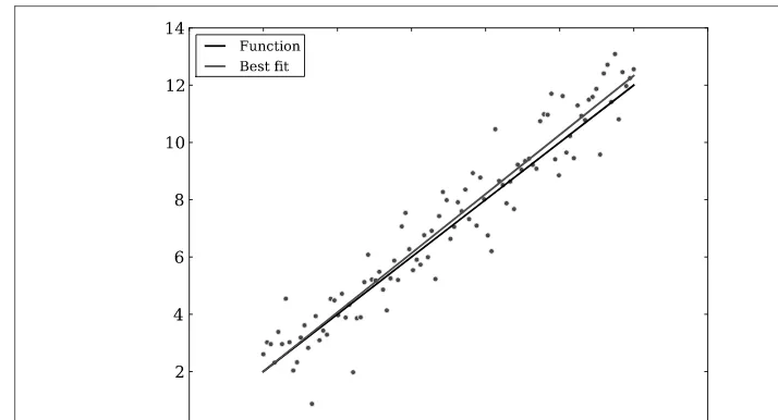
There are several ways to fit data with a linear regression. In this section we will use curve_fit, which is a χ2-based method (in other words, a best-fit method). In the example below, we generate data from a known function with noise, and then fit the noisy data withcurve_fit. The function we will model in the example is a simple linear equation,f (x)=ax+b.

from scipy.optimize import curve_fit

# Creating a function to model and create data def func(x, a, b):

return a * x + b

# Generating clean data x = np.linspace(0, 10, 100) y = func(x, 1, 2)

# Adding noise to the data

yn = y + 0.9 * np.random.normal(size=len(x))

# Executing curve_fit on noisy data popt, pcov = curve_fit(func, x, yn)

# popt returns the best fit values for parameters of # the given model (func).

print(popt)

The values frompopt, if a good fit, should be close to the values for theyassignment. You can check the quality of the fit withpcov, where the diagonal elements are the variances for each parameter. Figure 3-1 gives a visual illustration of the fit.

Taking this a step further, we can do a least-squares ﬁt to a Gaussian proﬁle, a non-linear function:

a_∗exp

−(x₋µ)2

2σ2

,

whereais a scalar,µis the mean, andσ is the standard deviation.

# Creating a function to model and create data def func(x, a, b, c):

return a*np.exp(-(x-b)**2/(2*c**2))

# Generating clean data x = np.linspace(0, 10, 100) y = func(x, 1, 5, 2)

(28)

Figure 3-1. Fitting noisy data with a linear equation.

Figure 3-2. Fitting noisy data with a Gaussian equation.

# popt returns the best-fit values for parameters of the given model (func). print(popt)

As we can see in Figure 3-2, the result from the Gaussian ﬁt is acceptable.

Going one more step, we can fit a one-dimensional dataset with multiple Gaussian profiles. Thefuncis now expanded to include two Gaussian equations with different input variables. This example would be the classic case of fitting line spectra (see Figure 3-3).

(29)

Figure 3-3. Fitting noisy data with multiple Gaussian equations.

# Two-Gaussian model

def func(x, a0, b0, c0, a1, b1,c1):

return a0*np.exp(-(x - b0) ** 2/(2 * c0 ** 2))\ + a1 * np.exp(-(x - b1) ** 2/(2 * c1 ** 2))

# Generating clean data x = np.linspace(0, 20, 200) y = func(x, 1, 3, 1, -2, 15, 0.5)

# Since we are fitting a more complex function, # providing guesses for the fitting will lead to # better results.

guesses = [1, 3, 1, 1, 15, 1] # Executing curve_fit on noisy data popt, pcov = curve_fit(func, x, yn, p0=guesses)

3.1.2 Solutions to Functions

With data modeling and ﬁtting under our belts, we can move on to ﬁnding solutions, such as “What is the root of a function?” or “Where do two functions intersect?” SciPy provides an arsenal of tools to do this in theoptimizemodule. We will run through the primary ones in this section.

(30)

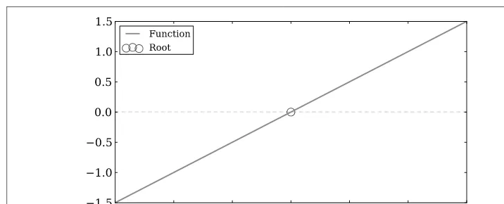
Figure 3-4. Approximate the root of a linear function aty=0.

from scipy.optimize import fsolve import numpy as np

line = lambda x: x + 3

solution = fsolve(line, -2) print solution

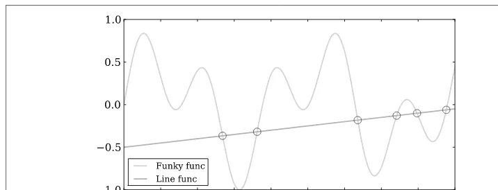
Finding the intersection points between two equations is nearly as simple.3 from scipy.optimize import fsolve

# Defining function to simplify intersection solution def findIntersection(func1, func2, x0):

return fsolve(lambda x : func1(x) - func2(x), x0)

# Defining functions that will intersect funky = lambda x : np.cos(x / 5) * np.sin(x / 2) line = lambda x : 0.01 * x - 0.5

# Defining range and getting solutions on intersection points x = np.linspace(0,45,10000)

result = findIntersection(funky, line, [15, 20, 30, 35, 40, 45])

# Printing out results for x and y print(result, line(result))

As we can see in Figure 3-5, the intersection points are well identiﬁed. Keep in mind that the assumptions about where the functions will intersect are important. If these are incorrect, you could get specious results.

3_{This is a modiﬁed example from}_{http://glowingpython.blogspot.de/2011/05/hot-to-find-intersection-of-two.html}_.

(31)

Figure 3-5. Finding the intersection points between two functions.

3.2 Interpolation

Data that contains information usually has a functional form, and as analysts we want to model it. Given a set of sample data, obtaining the intermediate values between the points is useful to understand and predict what the data will do in the non-sampled do-main. SciPy offers well over a dozen different functions for interpolation, ranging from those for simple univariate cases to those for complex multivariate ones. Univariate interpolation is used when the sampled data is likely led by one independent vari-able, whereas multivariate interpolation assumes there is more than one independent variable.

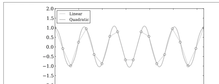
There are two basic methods of interpolation: (1) Fit one function to an entire dataset or (2) fit different parts of the dataset with several functions where the joints of each function are joined smoothly. The second type is known as a spline interpolation, which can be a very powerful tool when the functional form of data is complex. We will first show how to interpolate a simple function, and then proceed to a more complex case. The example below interpolates a sinusoidal function (see Figure 3-6) using scipy.interpolate.interp1dwith different fitting parameters. The first parameter is a “linear” fit and the second is a “quadratic” fit.

from scipy.interpolate import interp1d

# Setting up fake data

x = np.linspace(0, 10 * np.pi, 20) y = np.cos(x)

# Interpolating data

fl = interp1d(x, y, kind='linear') fq = interp1d(x, y, kind='quadratic')

# x.min and x.max are used to make sure we do not # go beyond the boundaries of the data for the # interpolation.

xint = np.linspace(x.min(), x.max(), 1000) yintl = fl(xint)

(32)

Figure 3-6. Synthetic data points (red dots) interpolated with linear and quadratic parameters.

Figure 3-7. Interpolating noisy synthetic data.

Figure 3-6 shows that in this case the quadratic ﬁt is far better. This should demonstrate how important it is to choose the proper parameters when interpolating data.

Can we interpolate noisy data? Yes, and it is surprisingly easy, using a spline-ﬁtting function calledscipy.interpolate.UnivariateSpline. (The result is shown in Figure 3-7.)

import matplotlib.pyplot as mpl

from scipy.interpolate import UnivariateSpline

# Setting up fake data with artificial noise sample = 30

x = np.linspace(1, 10 * np.pi, sample)

y = np.cos(x) + np.log10(x) + np.random.randn(sample) / 10

# Interpolating the data f = UnivariateSpline(x, y, s=1)

(33)

# x.min and x.max are used to make sure we do not # go beyond the boundaries of the data for the # interpolation.

xint = np.linspace(x.min(), x.max(), 1000) yint = f(xint)

The optionsis the smoothing factor, which should be used when ﬁtting data with noise. If insteads=0, then the interpolation will go through all points while ignoring noise.

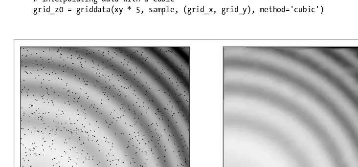
Last but not least, we go over a multivariate example—in this case, to reproduce an image. Thescipy.interpolate.griddatafunction is used for its capacity to deal with unstructuredN-dimensional data. For example, if you have a 1000×1000-pixel image, and then randomly selected 1000 points, how well could you reconstruct the image? Refer to Figure 3-8 to see how wellscipy.interpolate.griddata performs.

from scipy.interpolate import griddata

# Defining a function

ripple = lambda x, y: np.sqrt(x**2 + y**2)+np.sin(x**2 + y**2)

# Generating gridded data. The complex number defines # how many steps the grid data should have. Without the # complex number mgrid would only create a grid data structure # with 5 steps.

grid_x, grid_y = np.mgrid[0:5:1000j, 0:5:1000j]

# Generating sample that interpolation function will see xy = np.random.rand(1000, 2)

sample = ripple(xy[:,0] * 5 , xy[:,1] * 5)

# Interpolating data with a cubic

grid_z0 = griddata(xy * 5, sample, (grid_x, grid_y), method='cubic')

(34)

On the left-hand side of Figure 3-8 is the original image; the black points are the randomly sampled positions. On the right-hand side is the interpolated image. There are some slight glitches that come from the sample being too sparse for the ﬁner structures. The only way to get a better interpolation is with a larger sample size. (Note that thegriddatafunction has been recently added to SciPy and is only available for version 0.9 and beyond.)

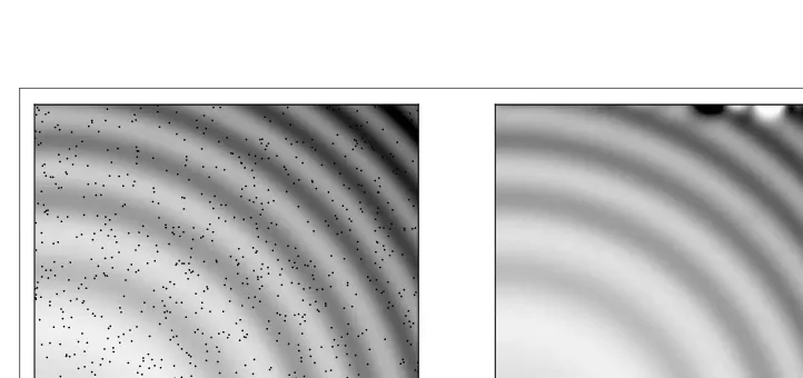
If we employ another multivariate spline interpolation, how would its results compare? Here we usescipy.interpolate.SmoothBivariateSpline, where the code is quite similar to that in the previous example.

from scipy.interpolate import SmoothBivariateSpline as SBS

# Defining a function

ripple = lambda x, y: np.sqrt(x**2 + y**2)+np.sin(x**2 + y**2)

# Generating sample that interpolation function will see xy= np.random.rand(1000, 2)

x, y = xy[:,0], xy[:,1]

sample = ripple(xy[:,0] * 5 , xy[:,1] * 5)

# Interpolating data

fit = SBS(x * 5, y * 5, sample, s=0.01, kx=4, ky=4)

interp = fit(np.linspace(0, 5, 1000), np.linspace(0, 5, 1000))

We have a similar result to that in the last example (Figure 3-9). The left panel shows the original image with randomly sampled points, and in the right panel is the interpolated data. TheSmoothBivariateSplinefunction appears to work a bit better thangriddata, with an exception in the upper-right corner.

Figure 3-9. Original image with random sample (black points, left) and the interpolated image (right).

(35)

Although from the ﬁgureSmoothBivariateSplinedoes appear to work better, run the code several times to see what happens. SmoothBivariate-Splineis very sensitive to the data sample it is given, and interpolations can go way off the mark.griddatais more robust and can produce a reasonable interpolation regardless of the data sample it is given.

3.3 Integration

Integration is a crucial tool in math and science, as differentiation and integration are the two key components of calculus. Given a curve from a function or a dataset, we can calculate the area below it. In the traditional classroom setting we would integrate a function analytically, but data in the research setting is rarely given in this form, and we need to approximate its deﬁnite integral.

The main purpose of integration with SciPy is to obtain numerical solu-tions. If you need indeﬁnite integral solutions, then you should look at SymPy.4It solves mathematical problems symbolically for many types of computation beyond calculus.

SciPy has a range of different functions to integrate equations and data. We will first go over these functions, and then move on to the data solutions. Afterward, we will employ the data-fitting tools we used earlier to compute definite integral solutions.

3.3.1 Analytic Integration

We will begin working with the function expressed below. It is straightforward to integrate and its solution’s estimated error is small. See Figure 3-10 for the visual context of what is being calculated.

3

0

cos2(ex)dx (3.1)

from scipy.integrate import quad

# Defining function to integrate func = lambda x: np.cos(np.exp(x)) ** 2

# Integrating function with upper and lower # limits of 0 and 3, respectively

solution = quad(func, 0, 3) print solution

# The first element is the desired value # and the second is the error.

# (1.296467785724373, 1.397797186265988e-09)

(36)

Figure 3-10. Definite integral (shaded region) of a function.

Figure 3-11. Definite integral (shaded region) of a function. The original function is the line and the randomly sampled data points are in red.

3.3.2 Numerical Integration

Let’s move on to a problem where we are given data instead of some known equation and numerical integration is needed. Figure 3-11 illustrates what type of data sample can be used to approximate acceptable indeﬁnite integrals.

from scipy.integrate import quad, trapz

# Setting up fake data

x = np.sort(np.random.randn(150) * 4 + 4).clip(0,5) func = lambda x: np.sin(x) * np.cos(x ** 2) + 1 y = func(x)

# Integrating function with upper and lower # limits of 0 and 5, respectively

fsolution = quad(func, 0, 5) dsolution = trapz(y, x=x)

(37)

print('fsolution = ' + str(fsolution[0])) print('dsolution = ' + str(dsolution))

print('The difference is ' + str(np.abs(fsolution[0] - dsolution)))

# fsolution = 5.10034506754 # dsolution = 5.04201628314

# The difference is 0.0583287843989.

Thequadintegrator can only work with a callable function, whereastrapzis a numerical integrator that utilizes data points.

3.4 Statistics

In NumPy there are basic statistical functions likemean,std,median,argmax, andargmin. Moreover, thenumpy.arrayshave built-in methods that allow us to use most of the NumPy statistics easily.

# Constructing a random array with 1000 elements x = np.random.randn(1000)

# Calculating several of the built-in methods # that numpy.array has

mean = x.mean() std = x.std() var = x.var()

For quick calculations these methods are useful, but more is usually needed for quan-titative research. SciPy offers an extended collection of statistical tools such as distribu-tions (continuous or discrete) and funcdistribu-tions. We will ﬁrst cover how to extrapolate the different types of distributions. Afterward, we will discuss the SciPy statistical functions used most often in various ﬁelds.

3.4.1 Continuous and Discrete Distributions

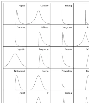
There are roughly 80 continuous distributions and over 10 discrete distributions. Twenty of the continuous functions are shown in Figure 3-12 as probability density functions (PDFs) to give a visual impression of what thescipy.statspackage provides. These distributions are useful as random number generators, similar to the functions found innumpy.random. Yet the rich variety of functions SciPy provides stands in con-trast to thenumpy.randomfunctions, which are limited to uniform and Gaussian-like distributions.

When we call a distribution fromscipy.stats, we can extract its information in several ways: probability density functions (PDFs), cumulative distribution functions (CDFs), random variable samples (RVSs), percent point functions (PPFs), and more. So how do we set up SciPy to give us these distributions? Working with the classic normal function

PDF=e(−x2/2)/

√

(38)

Figure 3-12. A sample of 20 continuous distributions in SciPy.

we demonstrate how to access the distribution.

import scipy.stats import norm

# Set up the sample range x = np.linspace(-5,5,1000)

(39)

# Here set up the parameters for the normal distribution, # where loc is the mean and scale is the standard deviation. dist = norm(loc=0, scale=1)

# Retrieving norm's PDF and CDF pdf = dist.pdf(x)

cdf = dist.cdf(x)

# Here we draw out 500 random values from the norm. sample = dist.rvs(500)

The distribution can be centered at a different point and scaled with the optionslocand scaleas shown in the example. This works as easily with all distributions because of their functional behavior, so it is important to read the documentation5when necessary. In other cases one will need a discrete distribution like the Poisson, binomial, or geo-metric. Unlike continuous distributions, discrete distributions are useful for problems where a given number of events occur in a ﬁxed interval of time/space, the events occur with a known average rate, and each event is independent of the prior event.

Equation 3.3 is the probability mass function (PMF) of the geometric distribution.

PMF=(1−p)(k−1)p (3.3)

from scipy.stats import geom

# Here set up the parameters for the geometric distribution. p = 0.5

dist = geom(p)

# Set up the sample range. x = np.linspace(0, 5, 1000)

# Retrieving geom's PMF and CDF pmf = dist.pmf(x)

cdf = dist.cdf(x)

# Here we draw out 500 random values. sample = dist.rvs(500)

3.4.2 Functions

There are more than 60 statistical functions in SciPy, which can be overwhelming to digest if you simply are curious about what is available. The best way to think of the statistics functions is that they either describe or test samples—for example, the frequency of certain values or the Kolmogorov-Smirnov test, respectively.

Since SciPy provides a large range of distributions, it would be great to take advantage of the ones we covered earlier. In thestatspackage, there are a number of functions

(40)

such askstestandnormaltestthat test samples. These distribution tests can be very helpful in determining whether a sample comes from some particular distribution or not. Before applying these, be sure you have a good understanding of your data, to avoid misinterpreting the functions’ results.

import numpy as np from scipy import stats

# Generating a normal distribution sample # with 100 elements

sample = np.random.randn(100)

# normaltest tests the null hypothesis. out = stats.normaltest(sample)

print('normaltest output') print('Z-score = ' + str(out[0])) print('P-value = ' + str(out[1]))

# kstest is the Kolmogorov-Smirnov test for goodness of fit. # Here its sample is being tested against the normal distribution. # D is the KS statistic and the closer it is to 0 the better. out = stats.kstest(sample, 'norm')

print('\nkstest output for the Normal distribution') print('D = ' + str(out[0]))

print('P-value = ' + str(out[1]))

# Similarly, this can be easily tested against other distributions, # like the Wald distribution.

out = stats.kstest(sample, 'wald')

print('\nkstest output for the Wald distribution') print('D = ' + str(out[0]))

print('P-value = ' + str(out[1]))

Researchers commonly use descriptive functions for statistics. Some descriptive func-tions that are available in thestatspackage include the geometric mean (gmean), the skewness of a sample (skew), and the frequency of values in a sample (itemfreq). Using these functions is simple and does not require much input. A few examples follow.

import numpy as np from scipy import stats

# Generating a normal distribution sample # with 100 elements

sample = np.random.randn(100)

# The harmonic mean: Sample values have to # be greater than 0.

out = stats.hmean(sample[sample > 0]) print('Harmonic mean = ' + str(out))

# The mean, where values below -1 and above 1 are # removed for the mean calculation

out = stats.tmean(sample, limits=(-1, 1)) print('\nTrimmed mean = ' + str(out))

(41)

# Calculating the skewness of the sample out = stats.skew(sample)

print('\nSkewness = ' + str(out))

# Additionally, there is a handy summary function called # describe, which gives a quick look at the data. out = stats.describe(sample)

print('\nSize = ' + str(out[0])) print('Min = ' + str(out[1][0])) print('Max = ' + str(out[1][1])) print('Mean = ' + str(out[2])) print('Variance = ' + str(out[3])) print('Skewness = ' + str(out[4])) print('Kurtosis = ' + str(out[5]))

There are many more functions available in thestatspackage, so the documentation is worth a look if you need more speciﬁc tools. If you need more statistical tools than are available here, try RPy.6 R is a cornerstone package for statistical analysis, and RPy ports the tools available in that system to Python. If you’re content with what is available in SciPy and NumPy but need more automated analysis, then take a look at Pandas.7It is a powerful package that can perform quick statistical analysis on big data. Its output is supplied in both numerical values and plots.

3.5 Spatial and Clustering Analysis

From biological to astrophysical sciences, spatial and clustering analysis are key to iden-tifying patterns, groups, and clusters. In biology, for example, the spacing of different plant species hints at how seeds are dispersed, interact with the environment, and grow. In astrophysics, these analysis techniques are used to seek and identify star clusters, galaxy clusters, and large-scale ﬁlaments (composed of galaxy clusters). In the computer science domain, identifying and mapping complex networks of nodes and information is a vital study all on its own. With big data and data mining, identifying data clusters is becoming important, in order to organize discovered information, rather than being overwhelmed by it.

If you need a package that provides good graph theory capabilities, check out NetworkX.8_{It is an excellent Python package for creating,} modu-lating, and studying the structure of complex networks (i.e., minimum spanning trees analysis).

SciPy provides a spatial analysis class (scipy.spatial) and a cluster analysis class (scipy.cluster). The spatial class includes functions to analyze distances between data points (e.g., k-d trees). The cluster class provides two overarching subclasses: vector quantization (vq) and hierarchical clustering (hierarchy). Vector quantization groups

(42)

large sets of data points (vectors) where each group is represented by centroids. The hierarchysubclass contains functions to construct clusters and analyze their substruc-tures.

3.5.1 Vector Quantization

Vector quantization is a general term that can be associated with signal processing, data compression, and clustering. Here we will focus on the clustering component, starting with how to feed data to thevqpackage in order to identify clusters.

from scipy.cluster import vq

# Creating data

c1 = np.random.randn(100, 2) + 5 c2 = np.random.randn(30, 2) - 5 c3 = np.random.randn(50, 2)

# Pooling all the data into one 180 x 2 array data = np.vstack([c1, c2, c3])

# Calculating the cluster centroids and variance # from kmeans

centroids, variance = vq.kmeans(data, 3)

# The identified variable contains the information # we need to separate the points in clusters # based on the vq function.

identified, distance = vq.vq(data, centroids)

# Retrieving coordinates for points in each vq # identified core

vqc1 = data[identified == 0] vqc2 = data[identified == 1] vqc3 = data[identified == 2]

The result of the identified clusters matches up quite well to the original data, as shown in Figure 3-13 (the generated cluster data is on the left and thevq-identified clusters are the on the right). But this was done only for data that had little noise. What happens if there is a randomly distributed set of points in the field? The algorithm fails with flying colors. See Figure 3-14 for a nice illustration of this.

3.5.2 Hierarchical Clustering

Hierarchical clustering is a powerful tool for identifying structures that are nested within larger structures. But working with the output can be tricky, as we do not get cleanly identiﬁed clusters like we do with thekmeanstechnique. Below is an example9

wherein we generate a system of multiple clusters. To employ the hierarchy function,

9_{The original effort in using this can be found at}

http://stackoverflow.com/questions/2982929/plotting-results-of-hierarchical-clustering-ontop-of-a-matrix-of-data-in-python.

(43)

Figure 3-13. Original clusters (left) andvq.kmeans-identified clusters (right). Points are associated to a cluster by color.

Figure 3-14. Original clusters (left) andvq.kmeans-identified clusters (right). Points are associated to a cluster by color. The uniformly distributed data shows the weak point of thevq.kmeansfunction.

we build a distance matrix, and the output is a dendrogram tree. See Figure 3-15 for a visual example of how hierarchical clustering works.

import matplotlib.pyplot as mpl from mpl_toolkits.mplot3d import Axes3D

from scipy.spatial.distance import pdist, squareform import scipy.cluster.hierarchy as hy

# Creating a cluster of clusters function

def clusters(number = 20, cnumber = 5, csize = 10):

# Note that the way the clusters are positioned is Gaussian randomness. rnum = np.random.rand(cnumber, 2)

rn = rnum[:,0] * number rn = rn.astype(int) rn[np.where(rn < 5 )] = 5

(44)

Figure 3-15. The pixelated subplot is the distance matrix, and the two dendrogram subplots show different types of dendrogram methods.

ra = rnum[:,1] * 2.9 ra[np.where(ra < 1.5)] = 1.5

cls = np.random.randn(number, 3) * csize

# Random multipliers for central point of cluster rxyz = np.random.randn(cnumber-1, 3)

for i in xrange(cnumber-1):

tmp = np.random.randn(rn[i+1], 3) x = tmp[:,0] + ( rxyz[i,0] * csize ) y = tmp[:,1] + ( rxyz[i,1] * csize ) z = tmp[:,2] + ( rxyz[i,2] * csize ) tmp = np.column_stack([x,y,z]) cls = np.vstack([cls,tmp]) return cls

(45)

# Generate a cluster of clusters and distance matrix. cls = clusters()

D = pdist(cls[:,0:2]) D = squareform(D)

# Compute and plot first dendrogram. fig = mpl.figure(figsize=(8,8)) ax1 = fig.add_axes([0.09,0.1,0.2,0.6]) Y1 = hy.linkage(D, method='complete') cutoff = 0.3 * np.max(Y1[:, 2])

Z1 = hy.dendrogram(Y1, orientation='right', color_threshold=cutoff) ax1.xaxis.set_visible(False)

ax1.yaxis.set_visible(False)

# Compute and plot second dendrogram. ax2 = fig.add_axes([0.3,0.71,0.6,0.2]) Y2 = hy.linkage(D, method='average') cutoff = 0.3 * np.max(Y2[:, 2])

Z2 = hy.dendrogram(Y2, color_threshold=cutoff) ax2.xaxis.set_visible(False)

# Plot distance matrix.

ax3 = fig.add_axes([0.3,0.1,0.6,0.6]) idx1 = Z1['leaves']

idx2 = Z2['leaves'] D = D[idx1,:] D = D[:,idx2]

ax3.matshow(D, aspect='auto', origin='lower', cmap=mpl.cm.YlGnBu) ax3.xaxis.set_visible(False)

# Plot colorbar.

fig.savefig('cluster_hy_f01.pdf', bbox = 'tight')

Seeing the distance matrix in the ﬁgure with the dendrogram tree highlights how the large and small structures are identiﬁed. The question is, how do we distinguish the structures from one another? Here we use a function calledfclusterthat provides us with the indices to each of the clusters at some threshold. The output fromfclusterwill depend on the method you use when calculating thelinkagefunction, such ascomplete

orsingle. The cutoff value you assign to the cluster is given as the second input in the fclusterfunction. In thedendrogramfunction, the cutoff’s default is0.7 * np.max(Y[:, 2]), but here we will use the same cutoff as in the previous example, with the scaler0.3.

# Same imports and cluster function from the previous example # follow through here.

# Here we define a function to collect the coordinates of # each point of the different clusters.

def group(data, index): number = np.unique(index) groups = []

for i in number:

groups.append(data[index == i])

(46)

# Creating a cluster of clusters cls = clusters()

# Calculating the linkage matrix

Y = hy.linkage(cls[:,0:2], method='complete')

# Here we use the fcluster function to pull out a # collection of flat clusters from the hierarchical # data structure. Note that we are using the same

# cutoff value as in the previous example for the dendrogram # using the 'complete' method.

cutoff = 0.3 * np.max(Y[:, 2])

index = hy.fcluster(Y, cutoff, 'distance')

# Using the group function, we group points into their # respective clusters.

groups = group(cls, index)

# Plotting clusters

fig = mpl.figure(figsize=(6, 6)) ax = fig.add_subplot(111)

colors = ['r', 'c', 'b', 'g', 'orange', 'k', 'y', 'gray'] for i, g in enumerate(groups):

i = np.mod(i, len(colors))

ax.scatter(g[:,0], g[:,1], c=colors[i], edgecolor='none', s=50) ax.xaxis.set_visible(False)

ax.yaxis.set_visible(False)

fig.savefig('cluster_hy_f02.pdf', bbox = 'tight')

The hierarchically identiﬁed clusters are shown in Figure 3-16.

Figure 3-16. Hierarchically identified clusters.

(47)

Figure 3-17. A stacked image that is composed of hundreds of exposures from the International Space Station.

3.6 Signal and Image Processing

SciPy allows us to read and write image files like JPEG and PNG images without worrying too much about the file structure for color images. Below, we run through a simple illustration of working with image files to make a nice image10(see Figure 3-17) from the International Space Station (ISS).

from scipy.misc import imread, imsave from glob import glob

# Getting the list of files in the directory files = glob('space/*.JPG')

# Opening up the first image for loop im1 = imread(files[0]).astype(np.float32)

# Starting loop and continue co-adding new images for i in xrange(1, len(files)):

print i

im1 += imread(files[i]).astype(np.float32)

# Saving img

imsave('stacked_image.jpg', im1)

10_{Original Pythonic effort can be found at}

(48)

Figure 3-18. A stacked image that is composed of hundreds