Modulation with Application to
Deep - Space Communications
Marvin K. Simon
MONOGRAPH 3
Issued by the Deep-Space Communications and Navigation Systems
Center of Excellence
Jet Propulsion Laboratory
California Institute of Technology
Joseph H. Yuen, Editor-in-Chief
Previously Published Monographs in this Series
1.
Radiometric Tracking Techniques for Deep-Space Navigation
C. L. Thornton and J. S. Border
2.
Formulation for Observed and Computed Values of
Deep Space Network Data Types for Navigation
Modulation with Application to
Deep-Space Communications
Marvin K. Simon
MONOGRAPH 3
DEEP–SPACE COMMUNICATIONS AND NAVIGATION SERIES
Jet Propulsion Laboratory
California Institute of Technology
With Technical Contributions by
Dennis Lee
Warren L. Martin
Haiping Tsou
Tsun-Yee Yan
(JPL Publication 00-17)
June 2001
v
Foreword
... vii
Preface
... ix
Chapter 1: Introduction
... 1
Chapter 2: Constant Envelope Modulations ... 3
2.1 The Need for Constant Envelope
... 3
2.2 Quadriphase-Shift-Keying and Offset (Staggered) Quadriphase-Shift-Keying
... 4
2.3 Differentially Encoded QPSK and Offset (Staggered) QPSK
... 8
2.4 π/4-QPSK: A Variation of Differentially Encoded QPSK with Instantaneous Amplitude Fluctuation Halfway between That of QPSK and OQPSK
... 9
2.5 Power Spectral Density Considerations
... 12
2.6 Ideal Receiver Performance
... 12
2.7 Performance in the Presence of Nonideal Transmitters
... 12
2.7.1
Modulator Imbalance and Amplifier Nonlinearity ... 12
2.7.2
Data Imbalance ... 26
2.8 Continuous Phase Modulation
... 26
2.8.1
Full Response—MSK and SFSK ... 27
2.8.2
Partial Response—Gaussian MSK ... 57
2.9 Simulation Performance
... 113
References
... 116
Chapter 3: Quasi-Constant Envelope Modulations
... 125
3.1 Brief Review of IJF-QPSK and SQORC and their Relation to FQPSK
... 129
3.2 A Symbol-by-Symbol Cross-Correlator Mapping for FQPSK
... 136
3.4 Interpretation of FQPSK as a Trellis-Coded
Modulation
... 146
3.5 Optimum Detection
... 147
3.6 Suboptimum Detection
... 152
3.6.1
Symbol-by-Symbol Detection ... 152
3.6.2
Average Bit-Error Probability Performance ... 159
3.6.3
Further Receiver Simplifications and FQPSK-B
Performance ... 161
3.7 Cross-Correlated Trellis-Coded Quadrature Modulation
... 166
3.7.1
Description of the Transmitter ... 168
3.7.2
Specific Embodiments ... 172
3.8 Other Techniques
... 177
3.8.1
Shaped Offset QPSK ... 177
References
... 184
Chapter 4: Bandwidth-Efficient Modulations with More Envelope Fluctuation
... 187
4.1 Bandwidth-Efficient TCM with Prescribed Decoding Delay—Equal Signal Energies
... 190
4.1.1
ISI-Based Transmitter Implementation ... 190
4.1.2
Evaluation of the Power Spectral Density ... 195
4.1.3
Optimizing the Bandwidth Efficiency ... 204
4.2 Bandwidth-Efficient TCM with Prescribed Decoding Delay—Unequal Signal Energies
... 212
References
... 218
Chapter 5: Strictly Bandlimited Modulations with Large Envelope Fluctuation (Nyquist Signaling)
... 219
5.1 Binary Nyquist Signaling
... 219
5.2 Multilevel and Quadrature Nyquist Signaling
... 223
References
... 223
Chapter 6: Summary
... 225
6.1 Throughput Performance Comparisons
... 225
vii
The Deep Space Communications and Navigation Systems Center of
Excellence (DESCANSO) was recently established for the National
Aeronau-tics and Space Administration (NASA) at the California Institute of
Technol-ogy’s Jet Propulsion Laboratory (JPL).
DESCANSO is chartered to harness
and promote excellence and innovation to meet the communications and
navi-gation needs of future deep-space exploration.
DESCANSO’s vision is to achieve continuous communications and precise
navigation—any time, anywhere. In support of that vision, DESCANSO aims
to seek out and advocate new concepts, systems, and technologies; foster key
scientific and technical talents; and sponsor seminars, workshops, and
sympo-sia to facilitate interaction and idea exchange.
The Deep Space Communications and Navigation Series, authored by
sci-entists and engineers with many years of experience in their respective fields,
lays a foundation for innovation by communicating state-of-the-art knowledge
in key technologies. The series also captures fundamental principles and
prac-tices developed during decades of deep-space exploration at JPL. In addition, it
celebrates successes and imparts lessons learned. Finally, the series will serve
to guide a new generation of scientists and engineers.
ix
Traditional modulation methods adopted by space agencies for
transmit-ting telecommand and telemetry data have incorporated subcarriers as a
sim-ple means of separating different data types as well ensuring no overlap
between the radio frequency (RF) carrier and the modulated data’s frequency
spectra. Unfortunately, subcarrier modulation suffers from a number of
disad-vantages, namely, greater spacecraft complexity, additional losses in the
mod-ulation/demodulation process, and most important, at least from the
standpoint of this monograph, a large, occupied bandwidth. One effort to
mit-igate the latter was to replace the more traditional square-wave subcarriers
with sine-wave carriers, but this was not considered to be an acceptable
solu-tion for all space-explorasolu-tion missions.
additional spectral pulse shaping to the latter now made it possible to transmit
messages at a high data rate while using a comparatively small bandwidth.
The purpose of this monograph is to define, describe, and then give the
performance (power and bandwidth) of digital communication systems that
incorporate a large variety of the bandwidth-efficient modulations referred to
above. In addition to considering the ideal behavior of such systems, we shall
also cover their performance in the presence of a number of practical
(non-ideal) transmitter and receiver characteristics such as modulator and phase
imbalance, imperfect carrier synchronization, and transmitter nonlinearity.
With regard to the latter, the requirement of operating the transmitter at a high
power efficiency, i.e., running the power amplifier in a saturated or
near-satu-rated condition, implies that one employ a constant envelope modulation.
This constraint restricts the type of modulations that can be considered, which
in turn restricts the amount of spectral occupancy and power efficiency that
can be achieved. Relaxing the constant envelope condition (which then allows
for a more linear but less efficient transmitter power amplifier operation)
potentially eases the restrictions on power and bandwidth efficiency to the
extreme limit of Nyquist-type signaling, which, in theory, is strictly
bandlim-ited and capable of achieving the maximum power efficiency. Because of this
inherent trade-off between envelope (or more correctly, instantaneous
ampli-tude) fluctuation of the modulation and the degree of power and bandwidth
efficiency attainable, we have chosen to structure this monograph in a way
that clearly reflects this issue. In particular, we start by discussing strictly
constant envelope modulations and then, moving in the direction of more and
more envelope fluctuation, end with a review of strictly bandlimited
(Nyquist-type) signaling. Along the way, we consider a number of
quasi-con-stant envelope modulations that have gained considerable notoriety in recent
years and represent a good balance among the above-mentioned power and
bandwidth trade-off considerations.
Finally, it should be mentioned that although the monograph attempts to
cover a large body of the published literature in this area, the real focus is on
the research and the results obtained at the Jet Propulsion Laboratory (JPL).
As such, we do not offer this document to the readership as an all-inclusive
treatise on the subject of bandwidth-efficient modulations but rather one that,
as the title reflects, highlights the many technical contributions performed
under NASA-funded tasks pertaining to the development and design of
deep-space communications systems. When taken in this context, we hope that, in
addition to being informative, this document will serve as an inspiration to
future engineers to continue the fine work that was initiated at JPL and has
been reported on herein.
Introduction
The United States Budget Reconciliation Act of 1993 mandates reallocation of a minimum of 200 MHz of spectrum below 5 GHz for licensing to nonfederal users. One of the objectives is to promote and encourage novel spectrum-inspired technology developments and wireless applications. Many user organizations and communications companies have been developing advanced modulation tech-niques in order to more efficiently use the spectrum.
In 1998, the international Space Frequency Coordination Group (SFCG) adopted a spectral mask that precludes the use of a number of classical modu-lation schemes for missions launched after 2002. The SFCG has recommended several advanced modulations that potentially could reduce spectrum conges-tion. No one technique solves every intended applicaconges-tion. Many trade-offs must be made in selecting a particular technique, the trade-offs being defined by the communications environment, data integrity requirements, data latency require-ments, user access, traffic loading, and other constraints. These new modulation techniques have been known in theory for many years, but have become feasible only because of recent advances in digital signal processing and microprocessor technologies.
This monograph focuses on the most recent advances in spectrum-efficient modulation techniques considered for government and commercial applications. Starting with basic, well-known digital modulations, the discussion will evolve to more sophisticated techniques that take on the form of constant envelope modulations, quasi-constant envelope modulations, nonconstant envelope mod-ulations, and finally Nyquist-rate modulations. Included in the discussion will be a unified treatment based on recently developed cross-correlated trellis-coded quadrature modulation (XTCQM), which captures a number of state-of-the-art spectrally efficient modulation schemes. Performance analysis, computer simula-tion results, and their hardware implicasimula-tions will be addressed. Comparisons of
Constant Envelope Modulations
2.1 The Need for Constant Envelope
Digital communication systems operate in the presence of path loss and atmospheric-induced fading. In order to maintain sufficient received power at the destination, it is required that a device for generating adequate transmitter output power based on fixed- but-limited available power be employed, exam-ples of which are traveling-wave tube amplifiers (TWTAs) and solid-state power amplifiers (SSPAs) operated in full- saturation mode to maximize conversion efficiency. Unfortunately, this requirement introduces amplitude modulation-amplitude modulation (AM-AM) and modulation-amplitude modulation-phase modulation (AM-PM) conversions into the transmitted signal. Because of this, modulations that transmit information via their amplitude, e.g., quadrature amplitude mod-ulation (QAM), and therefore need a linear amplifying characteristic, are not suitable for use on channels operated in the above maximum transmitter power efficiency requirement.1 Another consideration regarding radio frequency (RF) amplifier devices that operate in a nonlinear mode at or near saturation is the spectral spreading that they reintroduce due to the nonlinearity subsequent to bandlimiting the modulation prior to amplification. Because of the need for the transmitted power spectrum to fall under a specified mask imposed by regulat-ing agencies such as the FCC or International Telecommunications Union (ITU), the modulation must be designed to keep this spectral spreading to a minimum. This constraint necessitates limiting the amount of instantaneous amplitude fluc-tuation in the transmitted waveform in addition to imposing the requirement for constant envelope.
1
An approach whereby it might be possible to generate QAM-type modulations using separate nonlinearly operated high-power amplifiers on the inphase (I) and quadrature (Q) channels is currently under investigation by the author.
Because of the above considerations regarding the need for high transmit-ter power efficiency, it is clearly desirable to consider modulations that achieve their bandwidth efficiency by means other than resorting to multilevel amplitude modulation. Such constant envelope modulations are the subject of discussion in the first part of this monograph. Because of the large number of possible can-didates, to keep within the confines of a reasonable size book, we shall restrict our attention to only those that have some form of inphase-quadrature phase (I-Q) representation and as such an I-Q form of receiver.
2.2 Quadriphase-Shift-Keying and Offset (Staggered)
Quadriphase-Shift-Keying
M-ary phase-shift-keying (M-PSK) produces a constant envelope signal that is mathematically modeled in complexform2as
˜
s(t) =√2P ej(2πfct+θ(t)+θc)= ˜S(t)ej(2πfct+θc) (2.2 1)
where P is the transmitted power, fc is the carrier frequency in hertz, θc is
the carrier phase, andθ(t) is the data phase that takes on equiprobable values
βi = (2i−1)π/M, i= 1,2,· · ·, M, in each symbol interval,Ts. As such, θ(t) is
modeled as a random pulse stream, that is,
θ(t) =
∞
n=−∞
θnp(t−nTs) (2.2 2)
whereθnis the information phase in thenth symbol interval,nTs< t≤(n+1)Ts,
ranging over the set ofM possible valuesβias above, andp(t) is a unit amplitude
rectangular pulse of duration Ts seconds. The symbol time, Ts, is related to
the bit time, Tb, byTs =Tblog2M and, thus, the nominal gain in bandwidth
efficiency relative to binary phase-shift-keying (BPSK), i.e., M = 2, is a factor of log2M. The signal constellation is a unit circle with points uniformly spaced
by 2π/M rad. Thus, the complexsignal transmitted in the nth symbol interval is
˜
s(t) =√2P ej(2πfct+θn+θc), nT
s< t≤(n+ 1)Ts, n=−∞,· · ·,∞ (2.2 3)
2
Note that because of the assumed rectangular pulse shape, the complexbase-band signal ˜S(t) =√2P ejθn is constant in this same interval and has envelope
S˜(t)
=
√
2P.
A special case ofM-PSK that has an I-Q representation is quadriphase-shift-keying (QPSK), and corresponds to M = 4. Here it is conventional to assume that the phase set{βi} takes on valuesπ/4, 3π/4,5π/4,7π/4. Projecting these information phases on the quadrature amplitude axes, we can equivalently write QPSK in thenth symbol interval in the complexI-Q form3
˜
s(t) =√P(aIn+jaQn)ej(2πfct+θc), nTs< t≤(n+ 1)Ts (2.2 4)
where the information amplitudes aIn and aQn range independently over the
equiprobable values±1. Here again, because of the assumed rectangular pulse shape, the complexbaseband signal ˜S(t) =√P(aIn+jaQn) is constant in this
same interval. The real transmitted signal corresponding to (2.2-4) has the form
s(t) =√P mI(t) cos (2πfct+θc)− √
P mQ(t) sin (2πfct+θc),
mI(t) =
∞
n=−∞
aInp(t−nTs), mQ(t) =
∞
n=−∞
aQnp(t−nTs) (2.2 5)
If one examines the form of (2.2-4) it becomes apparent that a large fluctua-tion of the instantaneous amplitude between symbols corresponding to a 180-deg phase reversal can occur when both aIn and aQn change polarity at the same
time. As mentioned in Sec. 2.1, it is desirable to limit the degree of such fluc-tuation to reduce spectral regrowth brought about by the transmit amplifier nonlinearity, i.e., the smaller the fluctuation, the smaller the sidelobe regenera-tion and vice versa. By offsetting (staggering) the I and Q modularegenera-tions byTs/2 s,
one guarantees the fact that aIn and aQn cannot change polarity at the same
time. Thus, the maximum fluctuation in instantaneous amplitude is now limited to that corresponding to a 90-deg phase reversal (i.e., either aIn or aQn, but
not both, change polarity). The resulting modulation, called offset (staggered) QPSK (OQPSK), has a signal of the form
3
One can think of the complex carrier as being modulated now by a complex random pulse stream, namely, ˜a(t) =∞n=−∞
aIn+jaQn
s(t) =√P mI(t) cos (2πfct+θc)− √
P mQ(t) sin (2πfct+θc),
mI(t) =
∞
n=−∞
aInp(t−nTs), mQ(t) =
∞
n=−∞ aQnp
t−
n+1
2
Ts
(2.2 6)
While it is true that forM-PSK with M = 2mand man arbitrary integer,
the information phases can be projected on the I and Q coordinates and as such obtain, in principle, an I-Q transmitter representation, it should be noted that the number of possible I-Q amplitude pairs obtained from these projections ex-ceedsM. Consequently, decisions on the resulting I and Q multilevel amplitude signals at the receiver are not independent in that each pair of amplitude deci-sions does not necessarily render one of the transmitted phases. Therefore, for
M ≥8 it is not practical to viewM-PSK in an I-Q form.
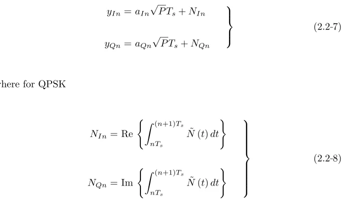
The detection of an information phase can be obtained by combining the detections on the I and Q components of this phase. The receiver for QPSK is illustrated in Fig. 2-1(a) while the analogous receiver for OQPSK is illustrated in Fig. 2-1(b). The decision variables that are input to the hard-limiting threshold devices are
yIn=aIn √
P Ts+NIn
yQn=aQn √
P Ts+NQn
(2.2 7)
where for QPSK
NIn = Re
(n+1)Ts
nTs
˜
N(t)dt
NQn= Im
(n+1)Ts
nTs
˜
N(t)dt
(2.2 8)
NIn = Re
(n+1)Ts
nTs
˜
N(t)dt
NQn= Im
(n+3/2)Ts
(n+1/2)Ts
˜
N(t)dt
(2.2 9)
In either case, NIn, NQn are zero mean Gaussian random variables (RVs) with
varianceσ2
N =N0Ts/2 and thus conditioned on the data symbols,yIn, yQn are
also Gaussian RVs with the same variance.
Fig. 2-1(a). Complex form of optimum receiver for ideal coherent detection of QPSK over the AWGN.
Received Carrier Oscillator
*
x (t) r(t)( )dt
(n+1) s nT s T
∫
1 Re { }yI n I Data Amplitude (Phase) Decision
a In
1 Im { }
yQ n Q Data Amplitude (Phase) Decision
a Qn cr(t) =e
j(2πfct+θc)
Fig. 2-1(b). Complex form of optimum receiver for ideal coherent detection of OQPSK over the AWGN.
Received Carrier Oscillator
cr(t) =e
j(2πfct+θc)
*
x(t)r(t)
yIn
I Data Amplitude (Phase) Decision
a In dt
(n+1)
s nT
∫
( )dt
∫
( ) Re { }
1
yQn
Q Data Amplitude (Phase) Decision
a Qn Im { }
1
(n+ )3 2 (n+ )1
2.3 Differentially Encoded QPSK and Offset (Staggered)
QPSK
In an actual coherent communication system transmittingM-PSK modula-tion, means must be provided at the receiver for establishing the local demodu-lation carrier reference signal. This means is traditionally accomplished with the aid of a suppressed carrier-tracking loop [1, Chap. 2]. Such a loop for M-PSK modulation exhibits an M-fold phase ambiguity in that it can lock with equal probability at the transmitted carrier phase plus any of theM information phase values. Hence, the carrier phase used for demodulation can take on any of these same M phase values, namely, θc+βi = θc + 2iπ/M, i = 0,1,2,· · ·, M −1.
Coherent detection cannot be successful unless this M-fold phase ambiguity is resolved.
One means for resolving this ambiguity is to employ differential phase en-coding (most often simply called differential enen-coding) at the transmitter and differential phase decoding (most often simply called differential decoding) at the receiver following coherent detection. That is, the information phase to be communicated is modulated on the carrier as the difference between two adjacent transmitted phases, and the receiver takes the difference of two adjacent phase decisions to arrive at the decision on the information phase.4 In mathematical
terms, if ∆θn were the information phase to be communicated in thenth
trans-mission interval, the transmitter would first form θn =θn−1+ ∆θn modulo 2π
(the differential encoder) and then modulateθn on the carrier.5 At the receiver,
successive decisions onθn−1andθnwould be made and then differenced modulo
2π(the differential decoder) to give the decision on ∆θn. Since the decision on
the true information phase is obtained from the difference of two adjacent phase decisions, a performance penalty is associated with the inclusion of differential encoding/decoding in the system.
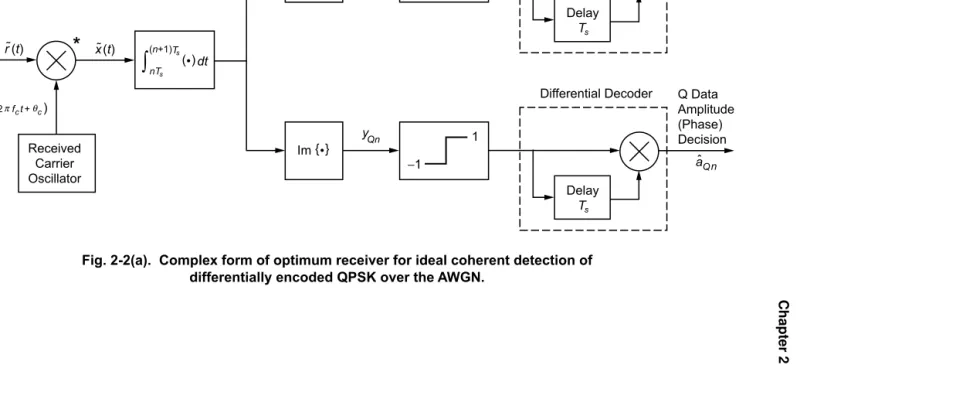
For QPSK or OQPSK, the differential encoding/decoding process can be performed on each of the I and Q channels independently. A block diagram of a receiver for differentially encoded QPSK (or OQPSK) would be identical to that shown in Fig. 2-1(a) [or Fig. 2-1(b)], with the inclusion of a binary differ-ential decoder in each of the I and Q arms following the hard-decision devices [see
4
Note that this receiver (i.e., the one that makes optimum coherent decisions on two successive symbol phases and then differences these to arrive at the decision on the information phase) is suboptimum whenM >2 [2]. However, this receiver structure, which is the one classically used for coherent detection of differentially encodedM-PSK, can be arrived at by a suitable approximation of the likelihood function used to derive the true optimum receiver, and at high signal-to-noise ratio (SNR), the difference between the two becomes mute.
5
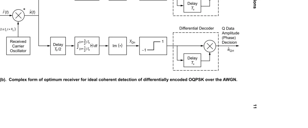
Figs. 2-2(a) and 2-2(b)].6 Inclusion of differentially encoded OQPSK in our
discussion is important since, as we shall see later on, other forms of modulation, e.g., minimum-shift-keying (MSK), have an I-Q representation in the form of pulse-shaped, differentially encoded OQPSK.
2.4
π
/4-QPSK: A Variation of Differentially Encoded QPSK
with Instantaneous Amplitude Fluctuation Halfway
between That of QPSK and OQPSK
Depending on the set of phases, {∆βi}, used to represent the information phase, ∆θn, in thenth transmission interval, the actual transmitted phase,θn, in
this same transmission interval can range either over the same set,{βi}={∆βi},
or over another phase set. If for QPSK, we choose the set ∆βi= 0, π/2, π,3π/2
to represent the information phases, then starting with an initial transmitted phase chosen from the set π/4, 3π/4,5π/4,7π/4, the subsequent transmit-ted phases, {θn}, will also range over the set π/4, 3π/4,5π/4,7π/4 in every transmission interval. This is the conventional form of differentially encoded QPSK, as discussed in the previous section. Now suppose instead that the set ∆βi = π/4,3π/4,5π/4,7π/4 is used to represent the information phases, {∆θn}. Then, starting, for example, with an initial phase chosen from the set π/4,3π/4,5π/4,7π/4, the transmitted phase in the next interval will range over the set 0, π/2, π,3π/2. In the following interval, the transmitted phase will range over the set π/4,3π/4,5π/4,7π/4, and in the interval following that one, the transmitted phase will once again range over the set 0, π/2, π,3π/2. Thus, we see that for this choice of phase set corresponding to the informa-tion phases,{∆θn}, the transmitted phases,{θn}, will alternatively range over
the sets 0, π/2, π,3π/2 and π/4,3π/4,5π/4,7π/4. Such a modulation scheme, referred to asπ/4-QPSK [3], has an advantage relative to conventional differen-tially encoded QPSK in that the maximum change in phase from transmission to transmission is 135 deg, which is halfway between the 90-deg maximum phase change of OQPSK and 180-deg maximum phase change of QPSK.
In summary, on a linear additive white Gaussian noise (AWGN) channel with ideal coherent detection, all three types of differentially encoded QPSK, i.e., con-ventional (nonoffset), offset, andπ/4 perform identically. The differences among the three types on a linear AWGN channel occur when the carrier demodulation phase reference is not perfect, which corresponds to nonideal coherent detection.
6
Since the introduction of a 180-deg phase shift to a binary phase sequence is equivalent to a reversal of the polarity of the binary data bits, a binary differential encoder is characterized byan=an−1bnand the corresponding binary differential decoder is characterized bybn= an−1anwhere{bn}are now the information bits and{an}are the actual transmitted bits
Chapter
2
Fig. 2-2(a). Complex form of optimum receiver for ideal coherent detection of differentially encoded QPSK over the AWGN.
Received Carrier Oscillator
*
x (t)( )dt s (n+1)
s nT
T
∫
Re { }
yIn
1
−1 Im { }
yQn cr(t) =e
j(2πfct+θc)
Differential Decoder
Delay
T s
1
−1
Differential Decoder
Delay
T s
I Data Amplitude (Phase) Decision
aIn
Q Data Amplitude (Phase) Decision
En
velope
Modulations
11
Fig. 2-2(b). Complex form of optimum receiver for ideal coherent detection of differentially encoded OQPSK over the AWGN.
Re { }
yIn
1
−1 Im { }
yQn
I Data Amplitude (Phase) Decision
aIn
Q Data Amplitude (Phase) Decision Differential Decoder
aQn
Delay
T s
1
−1
Differential Decoder
Delay
T s dt
(n+1)
s nT
s T
∫
( )Received Carrier Oscillator
cr(t) =e
j(2πfct +θc)
*
r(t) x(t)
( )dt
∫
(n+ )32
(n+ )1 2
Delay
s T/2
s T
2.5 Power Spectral Density Considerations
The power spectral densities (PSD) of QPSK, OQPSK, and the differentially encoded versions of these are all identical and are given by
S(f) =P Ts
sinπf T s
πf Ts 2
(2.5 1)
We see that the asymptotic (largef) rate of rolloff of the PSD varies asf−2, and
a first null (width of the main lobe) occurs atf = 1/Ts= 1/2Tb. Furthermore,
when compared with BPSK, QPSK is exactly twice as bandwidth efficient.
2.6 Ideal Receiver Performance
Based upon the decision variables in (2.2-7) the receiver for QPSK or OQPSK makes its I and Q data decisions from
ˆ
aIn= sgnyIn
ˆ
aQn= sgnyQn
(2.6 1)
which results in an average bit-error probability (BEP) given by
Pb(E) = 1
2erfc
Eb
N0
, Eb=P Tb (2.6 2)
and is identical to that of BPSK. Thus, we conclude that ideally BPSK, QPSK, and OQPSK have the identical BEP performance although the latter two occupy half the bandwidth.
2.7 Performance in the Presence of Nonideal Transmitters
2.7.1 Modulator Imbalance and Amplifier Nonlinearity
accurate average BEP performance. Here, we summarize some of these results for QPSK and OQPSK, starting with modulator imbalance acting alone and then later on in combination with amplifier nonlinearity. We begin our discus-sion with a description of an imbalance model associated with a modulator for generating these signals.
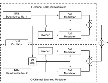
2.7.1.1 Modulator Imbalance Model. QPSK can be implemented with two balanced modulators, one on each of the I and Q channels, as illustrated in Fig. 2-3. Each of these modulators is composed of two AM modulators with inputs equal to the input nonreturn-to-zero (NRZ) data stream and its inverse (bit polarities inverted). The difference of the outputs of the two AM modula-tors serves as the BPSK transmitted signal on each channel. A mathematical description of the I and Q channel signals in the presence of amplitude and phase imbalances introduced by the AM modulators is7
sI(t) = √
P
2 mI(t)
cos (2πfct+θcI) + ΓIcos (2πfct+θcI+ ∆θcI)
+
√
P
2
cos (2πfct+θcI)−ΓIcos (2πfct+θcI+ ∆θcI) (2.7 1a)
sQ(t) = √
P
2 mQ(t)
sin (2πfct+θcQ) + ΓQsin (2πfct+θcQ+ ∆θcQ)
+
√
P
2
sin (2πfct+θcQ)−ΓQsin (2πfct+θcQ+ ∆θcQ) (2.7 1b)
s(t) =sI(t) +sQ(t)
where θcI, θcQ are the local oscillator carrier phases associated with the I and
Q balanced modulators, ΓI,ΓQ (both assumed to be less than unity) are the
relative amplitude imbalances of these same modulators, and ∆θcI,∆θcQ are
the phase imbalances between the two AM modulators in each of the I and Q
7
To be consistent with the usage in Ref. 8, we define the transmitted signal as the sum of the I and Q signals, i.e., s(t) =sI(t) +sQ(t) rather than their difference as in the more
AM Modulator
90 deg
Inverter NRZ
Data Source No. 1
Q-Channel Balanced Modulator I-Channel Balanced Modulator
Local Oscillator
AM Modulator
AM Modulator
AM Modulator Inverter
NRZ Data Source No. 2
Fig. 2-3. Balanced QPSK modulator implementation.
+ +
balanced modulators, respectively. Note that by virtue of the fact that we have introduced separate notation for the I and Q local oscillator phases, i.e.,θcI and
θcQ, we are also allowing for other than a perfect 90-deg phase shift between I and
Q channels. Alternatively, the model includes the possibility of an interchannel phase imbalance, ∆θc = θcI −θcQ. Since we will be interested only in the
difference ∆θc, without loss of generality we shall assume θcQ = 0, in which
case θcI = ∆θc. Finally, note that if ΓI = ΓQ = 1, ∆θcI = ∆θcQ = 0, and
θcI=θcQ=θc, then we obtain balanced QPSK as characterized by (2.2-5).
As shown in Ref. 8, the transmitted signal of (2.7-1a) and (2.7-1b) can, after some trigonometric manipulation, be written in the form
s(t) =√PαI +βImI(t)−γQ
1−mQ(t)
cos 2πfct
+αQ+βQmQ(t) +δI−γImI(t)
sin 2πfct
(2.7 2)
αI =
(1−ΓIcos ∆θcI) cos ∆θc+ ΓIsin ∆θcIsin ∆θc
2 ,
αQ=
1−ΓQcos ∆θcQ
2
βI =
(1 + ΓIcos ∆θcI) cos ∆θc−ΓIsin ∆θcIsin ∆θc
2 ,
βQ= 1 + ΓQcos ∆θcQ
2
γI = (1 + ΓIcos ∆θcI) sin ∆θc+ ΓIsin ∆θcIcos ∆θc
2 ,
γQ= ΓQsin ∆θcQ
2
δI = −(1−ΓIcos ∆θcI) sin ∆θc+ ΓIsin ∆θcIcos ∆θc
2
(2.7 3)
The form of the transmitted signal in (2.7-2) clearly identifies the crosstalk in-troduced by the modulator imbalances, i.e., the dependence of the I channel signal on the Q channel modulation and vice versa, as well as the lack of perfect quadrature between I and Q channels. Note the presence of a spurious carrier component in (2.7-3), i.e., a discrete (unmodulated) carrier component that is not present in the balanced case. Note that for perfect quadrature between the I and Q channels, i.e., ∆θc = 0, we haveγI =δI = (1/2)ΓIsin ∆θcI, and (2.7-2)
becomes the symmetric form
s(t) =√PαI+βImI(t)−γQ1−mQ(t)cos 2πfct
+αQ+βQmQ(t) +γI1−mI(t)sin 2πfct
(2.7 4)
which corresponds to the case of modulator imbalance alone. If now the phase imbalance is removed, i.e., ∆θcI = ∆θcQ = 0, then γI = γQ = 0, and the
of crosstalk at the receiver, which affects the system error probability perfor-mance. Finally, note that for the perfectly balanced case, βI = βQ = 1 and
αI =αI = 0, γI =γQ = 0, and (2.7-4) results in (2.2-5) with the exception of
the minus sign discussed in Footnote 7.
2.7.1.2 Effect on Carrier Tracking Loop Steady-State Lock Point.
When a Costas-type loop is used to track a QPSK signal, it forms its error signal fromIQI2−Q2, where the letters I and Q now refer to signals that are
synony-mous with the outputs of the inphase and quadrature integrate-and-dump (I&D) filters,yInandyQn, shown in Fig. 2-2(a). In the presence of modulator imbalance
and imperfect I and Q quadrature, the evaluation of the steady-state lock point of the loop was considered in Ref. 8 and, in the most general case, was determined numerically. For the special case of identically imbalanced I and Q modulators and no quadrature imperfection, i.e., ΓI = ΓQ = Γ, ∆θcI= ∆θcQ= ∆θu and
∆θc = 0, a closed-form result for the steady-state lock point is possible and is
given by
φ0=−14tan−1 6Γ
2sin 2∆θ
u+ Γ4sin 4∆θu
1 + 6Γ2cos 2∆θ
u+ Γ4cos 4∆θu
(2.7 5)
Note that for perfect modulator amplitude balance (Γ = 1), we obtain φ0 =
−∆θu/2, as expected. This shift in the lock point exists independently of the
loop SNR and thus can be referred to as an irreducible carrier phase error.
2.7.1.3 Effect on Average BEP. Assuming that the phase error is constant over the bit time (equivalently, the loop bandwidth is small compared to the data rate) and that the 90-deg phase ambiguity associated with the QPSK Costas loop can be perfectly resolved (e.g., by differential encoding), the average BEP can be evaluated by averaging the conditional (on the phase error,φ) BEP over the probability density function (PDF) of the phase error, i.e.,
PbI(E) =
φ0−π/4
φ0−π/4
PbI(E;φ)pφ(φ)dφ
PbQ(E) =
φ0−π/4
φ0−π/4
PbQ(E;φ)pφ(φ)dφ
(2.7 6)
where
pφ(φ) = 4
expρ4φcos4 (φ−φ0)
2πI0(ρ4φ)
, |φ−φ0| ≤ π
is the usual Tikhonov model assumed for the phase error PDF [11] with φ0
determined from (2.7-5). The parameterρ4φ is the loop SNR of the four times
phase error process (which is what the loop tracks) and I0(·) is the modified first-order Bessel function of the first kind. Based on the hard decisions made on
yIn andyQnin Fig. 2-2(a), the conditional BEPs on the I and Q channels in the
presence of imbalance are given, respectively, in Ref. 8, Eqs. (11a) and (11b):
PbI(E;φ) =
1 8erfc
Eb
N0
cos (φ+ ∆θc) + sinφ
+1 8erfc
Eb
N0
cos (φ+ ∆θc)−ΓQsin (φ+ ∆θcQ)
+1 8erfc
Eb
N0
ΓIcos (φ+ ∆θcI+ ∆θc)−sinφ
+1 8erfc
Eb
N0
ΓIcos (φ+ ∆θcI+ ∆θc) + ΓQsin (φ+ ∆θcQ)
(2.7 8a)
and
PbQ(E;φ) =
1 8erfc
Eb
N0
cosφ−sin (φ+ ∆θc)
+1 8erfc
Eb
N0
cosφ+ ΓIsin (φ+ ∆θcI+ ∆θc)
+1 8erfc
Eb
N0
ΓQcos (φ+ ∆θcQ) + sin (φ+ ∆θc)
+1 8erfc
Eb
N0
ΓQcos (φ+ ∆θcQ)−ΓIsin (φ+ ∆θcI+ ∆θc)
Substituting (2.7-7) together with (2.7-8a) and (2.7-8b) in (2.7-6) gives the de-sired average BEP of the I and Q channels for any degree of modulator imbalance. Note that, in general, the error probability performances of the I and Q channels are not identical.
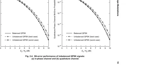
For a maximum amplitude imbalance (ΓI or ΓQ) of 0.2 dB, a maximum
phase imbalance (∆θcI or ∆θcQ) of +2 deg, and a maximum I-Q
quadra-ture imbalance (∆θc) of +2 deg (the values recommended by the CCSDS),
Figs. 2-4(a) and 2-4(b) plot the I and Q average BEPs as computed from (2.7-6) for the best and worst combinations of imbalance conditions. In these plots, the loop SNR,ρ4φ, is assumed to have infinite value (“perfect” carrier
synchroniza-tion), and, consequently, the degradation corresponds only to the shift in the lock point. The case of perfectly balanced QPSK is also included in these plots for comparison purposes. We observe that the best imbalance condition gives a performance virtually identical to that of balanced QPSK, whereas the worst imbalance condition results in an Eb/N0 loss of 0.33 dB at an average BEP of
10−2.
The extension of the above results to the case of OQPSK is presented in Ref. 9. The same modulator imbalance model as that illustrated in Fig. 2-3 is considered, with the exception that the Q channel data stream is now offset with respect to the I channel data stream, requiring a half-symbol delay between the NRZ data source 2 and AM modulator. Also, the amplitude imbalance, Γ, between the I and Q channels, is now explicitly included as an additional independent parameter. Therefore, analogous to (2.7-1b), the Q component of the transmitted OQPSK signal becomes [the I component is still given by (2.7-1a)]
sQ(t) = Γ √
P
2 mQ
t−T2s
sin (2πfct+θcQ) + ΓQsin (2πfct+θcQ+ ∆θcQ)
+ Γ
√
P
2
sin (2πfct+θcQ)−ΓQsin (2πfct+θcQ+ ∆θcQ) (2.7 9)
Using similar trigonometric manipulations for arriving at (2.7-2), the transmitted signal (sI(t) +sQ(t)) can now be written as
s(t) =√P
αI+βImI(t)−γQ
1−mQ
t−T2s
cos 2πfct
+
αQ+βQmQ
t−T2s
+δI−γImI(t)
sin 2πfct
En
velope
Modulations
19
0 1 2 3 4 5 6 7 8 9 10 Unbalanced QPSK (worst case)
Unbalanced QPSK (best case) Balanced QPSK
Eb / N0(dB)
Fig. 2-4. Bit-error performance of imbalanced QPSK signals: (a) in-phase channel and (b) quadrature channel.
In-Phase Channel Bit-Error Probability
10−6 10−5 10−4 10−3 10−2 10−1
0 1 2 3 4 5 6 7 8 9 10 Unbalanced QPSK (worst case)
Unbalanced QPSK (best case) Balanced QPSK
Eb / N0(dB)
Quadrature-Phase Channel Bit-Error Probability
10−6 10−5 10−4 10−3 10−2 10−1
where the only changes in the parameters of (2.7-3) are thatαQ, βQ, andγQ are
now each multiplied by the I-Q amplitude imbalance parameter, Γ.
The carrier-tracking loop assumed in Ref. 9 is a slightly modified version of that used for QPSK, in which a half-symbol delay is added to its I arm so that the symbols on both arms are aligned in forming theIQQ2−I2error signal. This
loop as well as the optimum (based on maximum a posteriori (MAP) estimation) OQPSK loop, which exhibits only a 180-deg phase ambiguity, are discussed in Ref. 12. The evaluation of the steady-state lock point of the loop was considered in Ref. 9 and was determined numerically. The average BEP is still determined from (2.7-6) (again assuming perfect 90-deg phase ambiguity resolution), but the conditional I and Q BEPs are now specified by
PbI(E;φ) =
1 16erfc
Eb
N0
cos (φ+ ∆θc) + sinφ
+ 1 16erfc
Eb
N0
cos (φ+ ∆θc)−ΓΓQsin (φ+ ∆θcQ)
+ 1 16erfc
Eb
N0
ΓIcos (φ+ ∆θcI+ ∆θc)−Γ sinφ
+ 1 16erfc
Eb
N0
ΓIcos (φ+ ∆θcI+ ∆θc) + ΓΓQsin (φ+ ∆θcQ)
+1 8erfc
Eb
N0
cos (φ+ ∆θc)−ΓΓQ
2 sin (φ+ ∆θcQ) + Γ 2 sinφ
+1 8erfc
Eb
N0
ΓIcos (φ+ ∆θcI+ ∆θc) +
ΓΓQ
2 sin (φ+ ∆θcQ)− Γ 2 sinφ
(2.7 11a)
PbQ(E;φ) =
1 16erfc
Eb
N0
Γ cosφ−sin (φ+ ∆θc)
+ 1 16erfc
Eb
N0
Γ cosφ+ ΓIsin (φ+ ∆θcI+ ∆θc)
+ 1 16erfc
Eb
N0
ΓΓQcos (φ+ ∆θcQ) + sin (φ+ ∆θc)
+ 1 16erfc
Eb
N0
ΓΓQcos (φ+ ∆θcQ)−ΓIsin (φ+ ∆θcI+ ∆θc)
+1 8erfc
Eb
N0
Γ cosφ+ΓI
2 sin (φ+ ∆θcI+ ∆θc) + 1
2sin (φ+ ∆θc)
+1 8erfc
Eb
N0
ΓΓQcos (φ+ ∆θcQ)−
ΓI
2 sin (φ+ ∆θcI+ ∆θc)
+1
2sin (φ+ ∆θc)
(2.7 11b)
Substituting (2.7-7) together with (2.7-11a) and (2.7-11b) in (2.7-6) gives the desired average BEP of the I and Q channels for any degree of modulator im-balance. Note again that, in general, the error probability performances of the I and Q channels are not identical.
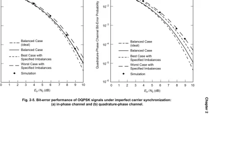
For the same maximum amplitude imbalance, maximum phase imbalance, and maximum I-Q quadrature imbalances as for the QPSK case and in addi-tion an I-Q amplitude imbalance (Γ) of −0.2 dB (corresponding to an actual Q-channel power that is 0.4 dB less than that in the I channel), Figs. 2-5(a) and 2-5(b) plot the I and Q average BEPs as computed from (2.7-6) for the best and worst combinations of imbalance conditions. These results also include the effect of a finite loop SNR of theφprocess,ρφ=ρ4φ/16, which was chosen equal
Chapter
2
Fig. 2-5. Bit-error performance of OQPSK signals under imperfect carrier synchronization: (a) in-phase channel and (b) quadrature-phase channel.
10−6 10−5 10−4 10−3 10−2 10
0 1 2
Eb / N0(dB)
3 4 5 6 7 8 9 10
In-Phase Channel Bit-Error Probability
Balanced Case
Simulation Balanced Case (ideal)
Best Case with Specified Imbalances Worst Case with Specified Imbalances
10−6 10−5 10−4 10−3 10−2 10
0 1 2
Eb / N0(dB)
3 4 5 6 7 8 9 10
Quadrature-Phase Channel Bit-Error Probability
Balanced Case
Simulation Balanced Case (ideal)
Best Case with Specified Imbalances Worst Case with Specified Imbalances
balanced QPSK (ideal) refers to the case where the loop SNR is assumed infinite, as was the case shown in Figs. 2-4(a) and 2-4(b). Finally, simulation points that agree with the analytical results are also included in Figs. 2-5(a) and 2-5(b). We observe from these figures that the worst imbalance condition results in an
Eb/N0 loss of 0.61 dB for the I channel and 1.08 dB for the Q-channel at an
average BEP of 10−4, the larger loss for the Q channel coming as a result of
its 0.4-dB power deficiency caused by the I-Q amplitude imbalance. When the I and Q results are averaged, the overallEb/N0degradation becomes 0.86 dB. If
perfect carrier synchronization had been assumed, then as shown in Ref. 9, these worst-case losses would be reduced to 0.34 dB for the I channel and 0.75 dB for the Q channel, which translates to a 0.58-dB average performance degradation. Aside from intrachannel and interchannel amplitude and phase imbalances, the inclusion of a fully saturated RF amplifier modeled by a bandpass hard lim-iter in the analytical model causes additional degradation in system performance. The performance of OQPSK on such a nonlinear channel was studied in Ref. 10, using the same modulator imbalance model as previously discussed above. The results are summarized as follows.
The transmitter is the same as that illustrated in Fig. 2-3 (with the inclusion of the half-symbol delay in the Q channel as previously discussed), the output of which is now passed through a nonlinear amplifier composed of the cascade of a hard limiter and a bandpass filter (a bandpass hard limiter [13]). The hard limiter clips its input signal at levels ±√2P1(π/4), and the bandpass (zonal) filter removes all the harmonics except for the one at the carrier frequency. The resulting bandpass hard-limited OQPSK signal is a constant envelope signal that has the form
ˆ
s(t) =2P1cos2πfct+θd(t)
(2.7 12)
whereP1=Pβ2
I +γI2
withβI, γI as defined in (2.7-3) and8
θd(t) = tan−1
γI
βI−
tan−1
GmQ
t−T2s
cos ∆θ+Acosψ
mI(t) +GmQ
t−T2s
sin ∆θ+Asinψ
(2.7 13)
with
8
G=
$ β2
Q+γQ2
β2
I +γI2
A=
$
(αI−γQ)2+ (αQ+δI)2
β2
I +γI2
∆θ= tan−1 γQ
βQ −
tan−1γI
βI
ψ= tan−1αI−γQ
αQ+δI −tan
−1γI
βI
(2.7 14)
Since in any half symbol interval, mI(t) andmQ(t−[Ts/2]) only take on
val-ues±1, then in that same interval,θd(t) takes on only one of four equiprobable
values, namely,θ1,1, θ−1,1, θ1,−1, θ−1,−1, where the subscripts correspond,
respec-tively, to the values of the above two modulations.
The average BEP is again computed from (2.7-6) together with (2.7-7), where the conditional BEPs are now given by [10, Eqs. (10a) and (10b)]
PbI(E;φ) =
1 2erfc
$
2E′
b
N0 cos
θd(1)−θ(2)d
2 cos
θ(1)d +θd(2)
2 +φ
(2.7 15)
PbQ(E;φ) = 1
2erfc
$
2E′
b
N0 cos
θd(2)−θ(3)d
2 cos
θ(2)d +θd(3)
2 +φ
where θ(dj) is the value of the symbol phase θd(t) in the interval (j−1)Ts/2≤
t≤jTs/2, the overbar denotes the statistical average over these symbol phases,
and E′
b = P1T /2Ts =β2I +γI2
P Ts/2 = βI2+γI2
Eb is the actual I-channel
Fig. 2-6. Bit-error performance of nonlinear OQPSK links with imperfect carrier synchronization (i.e., with a carrier-tracking loop SNR fixed at 22 dB): (a) overall channel, (b) in-phase channel, and (c) quadrature-phase channel.
10−6 10−5 10−4 10−3 10−2 10−1
10−6 10−5 10−4 10−3 10−2 10−1 10−6
10−5 10−4 10−3 10−2 10−1
Eb / N0 (dB)
Eb / N0 (dB)
Eb / N0 (dB)
In-Phase Channel Bit-Error Probability
0 1 2 3 4 5 6 7 8 9 10
0 1 2 3 4 5 6 7 8 9 10
0 1 2 3 4 5 6 7 8 9 10
Quadrature-Phase Channel Bit-Error Probability
(c)
A
verage Bit-Error Probability
(a)
Balanced Case (ideal)
Best Case with Specified Imbalances
Worst Case with Specified Imbalances Balanced Case
(ideal)
Best Case with Specified Imbalances
Worst Case with Specified Imbalances
Balanced Case (ideal)
Best Case with Specified Imbalances
Worst Case with Specified Imbalances
between the I and Q channels is itself more balanced. Furthermore, the average BEPs themselves are much closer to that of a perfectly balanced OQPSK system than those found for the linear channel.
2.7.2 Data Imbalance
The presence of data imbalance (positive and negative bits have different a priori probabilities of occurrence) in the transmitted waveform results in the addition of a discrete spectral component at dc to the continuous PSD component described by (2.5-1). Specifically, if pdenotes the probability of a mark (+1), then the total PSD is given by [11, Eq. (1-19)]
S(f) =P Ts
1
Ts
(1−2p)2δ(f) + 4p(1−p)sin
2πf T
s
(πf Ts)2
(2.7 16)
Clearly, for the balanced data case, i.e., p = 1/2, (2.7-16) reduces to (2.5-1). Since the total power in the transmitted signal is now split between an unmod-ulated tone at the carrier frequency and a data-bearing component, the carrier tracking process at the receiver (which is designed to act only on the latter) becomes affected even with perfect modulator balance. The degrading effects of a residual carrier on the Costas loop performance for binary PSK are discussed in Ref. 14. The extension to QPSK and OQPSK modulations is straightforward and not pursued here.
Further on in this monograph in our discussion of simulation models and performance, we shall talk about various types of filtered QPSK (which would then no longer be constant envelope). At that time, we shall observe that the combination of data imbalance and filtering produces additional discrete spectral harmonics occurring at integer multiples of the symbol rate.
2.8 Continuous Phase Modulation
CPM schemes are classified as being full response or partial response, de-pending, respectively, on whether the modulating frequency pulse is of a single bit duration or longer. Within the class of full response CPMs, the subclass of schemes having modulation index0.5 but arbitrary frequency pulse shape results in a form of generalized MSK [16].9 Included as popular special cases
are MSK, originally invented by Doelz and Heald, as disclosed in a 1961 U.S. patent [19], having a rectangular frequency pulse shape, and Amoroso’s sinu-soidal frequency-shift-keying (SFSK) [20], possessing a sinusinu-soidal (raised cosine) frequency pulse shape. The subclass of full-response schemes with rectangular frequency pulse but arbitrary modulation indexis referred to as continuous phase frequency-shift-keying (CPFSK) [21], which, for all practical purposes, served as the precursor to what later became known as CPM itself. Within the class of partial-response CPMs, undoubtedly the most popular scheme is that of Gaus-sian minimum-shift-keying (GMSK) which, because of its excellent bandwidth efficiency, has been adopted as a European standard for personal communication systems (PCSs). In simple terms, GMSK is a partial-response CPM scheme ob-tained by filtering the rectangular frequency pulses characteristic of MSK with a filter having a Gaussian impulse response prior to frequency modulation of the carrier.
In view of the above considerations, in what follows, we shall focus our CPM discussion only on MSK, SFSK, and GMSK, in each case presenting results for their spectral and power efficiency behaviors. Various representations of the transmitter, including the all-important equivalent I-Q one, will be discussed as well as receiver performance, both for ideal and nonideal (modulator imbalance) conditions.
2.8.1 Full Response—MSK and SFSK
While the primary intent of this section of the monograph is to focus specif-ically on the properties and performance of MSK and SFSK in the form they are most commonly known, the reader should bear in mind that many of these very same characteristics, e.g., transmitter/receiver implementations, equivalent I-Q signal representations, spectral and error probability analysis, apply equally well to generalized MSK. Whenever convenient, we shall draw attention to these analogies so as to alert the reader to the generality of our discussions. We begin the mathematical treatment by portraying MSK as a special case of the more general CPM signal, whose characterization is given in the next section.
9
2.8.1.1 Continuous Phase Frequency Modulation Representation. A binary single-mode (one modulation indexfor all transmission intervals) CPM signal is a constant envelope waveform that has the generic form (see the imple-mentation in Fig. 2-7)
s(t) =
2Eb
Tb cos
2πfct+φ(t,α) +φ0, nTb≤t≤(n+ 1)Tb (2.8 1)
where, as before,EbandTbrespectively denote the energy and duration of a bit
(P = Eb/Tb is the signal power), and fc is the carrier frequency. In addition,
φ(t,α) is the phase modulation process that is expressable in the form
φ(t,α) = 2π
i≤n
αihq(t−iTb) (2.8 2)
where α = (· · ·, α−2, α−1, α0, α1, α2,· · ·) is an independent, identically dis-tributed (i.i.d.) binary data sequence, with each element taking on equiprobable values±1,h= 2∆f Tb is the modulation index(∆f is the peak frequency
devi-ation of the carrier), andq(t) is the normalized phase-smoothing response that defines how the underlying phase, 2παih, evolves with time during the associated
bit interval. Without loss of generality, the arbitrary phase constant,φ0, can be set to zero.
For our discussion here it is convenient to identify the derivative of q(t), namely,
g(t) =dq(t)
dt (2.8 3)
Fig. 2-7. CPM transmitter.
Frequency Modulator Frequency
Pulse Shaping
g (t)
s (t) 2πh
fc
{αn }
α
ng (t− nTb)
Σ
n = − δ (t− nT)
which represents the instantaneous frequency pulse (relative to the nominal car-rier frequency,fc) in the zeroth signaling interval. In view of (2.8-3), the phase
smoothing response is given by
q(t) =
t
−∞
g(τ)dτ (2.8 4)
which, in general, extends over infinite time. For full response CPM schemes, as will be the case of interest here,q(t) satisfies the following:
q(t) =
0, t≤0 1
2, t≥Tb
(2.8 5)
and, thus, the frequency pulse, g(t), is nonzero only over the bit interval, 0≤t≤Tb. In view of (2.8-5), we see that theith data symbol,αi, contributes
a phase change ofπαihrad to the total phase for all time afterTb seconds of its
introduction, and, therefore, this fixed phase contribution extends over all fu-ture symbol intervals. Because of this overlap of the phase smoothing responses, the total phase in any signaling interval is a function of the present data sym-bol as well as all of the past symsym-bols, and accounts for the memory associated with this form of modulation. Consequently, in general, optimum detection of CPM schemes must be performed by a maximum-likelihood sequence estimator (MLSE) form of receiver [1] as opposed to bit-by-bit detection, which is optimum for memoryless modulations such as conventional binary FSK with discontinuous phase.
As previously mentioned, MSK is a full-response CPM scheme with a modu-lation indexh= 0.5 and a rectangular frequency pulse mathematically described by
g(t) =
1 2Tb
, 0≤t≤Tb
0, otherwise
(2.8 6)
For SFSK, one of the generalized MSK schemes mentioned in the introduction,
g(t), would be a raised cosine pulse given by
g(t) =
1 2Tb
1−cos
2πt Tb
, 0≤t≤Tb
0, otherwise
The associated phase pulses defined by (2.8-4) are
q(t) =
t
2Tb
, 0≤t≤Tb
1
2, t≥Tb
(2.8 8)
for MSK and
q(t) =
1 2Tb
t−sin 22π/Tπt/Tb b
, 0≤t≤Tb
1
2, t≥Tb
(2.8 9)
for SFSK.
Finally, substituting h = 0.5 and g(t) of (2.8-6) in (2.8-1) combined with (2.8-2) gives the CPM representations of MSK and SFSK, respectively, as
sMSK(t) =
2Eb
Tb
cos
2πfct+
π
2Tb
i≤n
αi(t−iTb)
, nTb≤t≤(n+ 1)Tb
(2.8 10)
and
sSFSK(t) =
2Eb
Tb
cos
2πfct+ π
2Tb
i≤n
αi
t−iTb−sin 2π(t−iTb)/Tb
2π/Tb
,
nTb ≤t≤(n+ 1)Tb (2.8 11)
both of which are implemented as in Fig. 2-7, usingg(t) of (2.8-6) or (2.8-7) as appropriate.
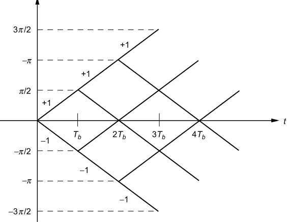
Associated with MSK (or SFSK) is a phase trellis that illustrates the evo-lution of the phase process with time, corresponding to all possible transmitted sequences. For MSK, the phase variation with time is linear [see (2.8-10)], and, thus, paths in the phase trellis are straight lines with a slope of±π/2Tb.
Fig. 2-8. Phase trellis (time-varying) for conventional MSK. Phase states (mod 2 ) are (0, ) for n even and ( /2, 3 /2) for n odd.
−π 3 π/2
−π /2 −π
/2 π
−3 π /2
t +1
−1
+1
+1
−1
2Tb
Tb 3Tb 4Tb
−1
π π π π
the change in phase over a single bit time is eitherπ/2 or−π/2, depending on the polarity of the data bit,αi, corresponding to that bit time. Also note that the
trellis is time-varying in that the phase states (modulo 2π) alternate between 0 andπat even multiples of the bit time andπ/2 and 3π/2 at odd multiples of the bit time. For SFSK, the phase trellis would appear as in Fig. 2-8 with, however, a sinusoidal variation in phase superimposed over the straight line paths. Here again the change in phase over a single bit time would be either π/2 or −π/2, depending on the polarity of the data bit,αi, corresponding to that bit time.
φ(t,α) = π 2Tb
i≤n
αi(t−iTb) =αn
π
2Tb(t−nTb) +
π
2
i≤n−1
αi=αn
π
2Tbt+xn,
nTb ≤t≤(n+ 1)Tb (2.8 12)
where (π/2)i≤n−1αi is the accumulated phase at the beginning of the nth
transmission interval that is equal to an odd integer (positive or negative) mul-tiple of π/2 when n is odd and an even integer (positive or negative) multiple of π/2 when n is even, and xn is a phase constant required to keep the phase
continuous at the data transition pointst =nTb andt = (n+ 1)Tb. Note also
thatxn represents they-intercept (when reduced modulo 2π) of the path in the
phase trellis that represents φ(t,α). In the previous transmission interval, the excess phase is given by
φ(t,α) =αn
π
2Tb
t−(n−1)Tb
+π 2
i≤n−2
αi=αn−1 π
2Tb
t+xn−1,
(n−1)Tb≤t≤nTb (2.8 13)
For phase continuity att=nTb, we require that
αn π
2Tb
(nTb) +xn=αn−1 π
2Tb
(nTb) +xn−1 (2.8 14)
or equivalently
xn=xn−1+ πn
2 (αn−1−αn) (2.8 15)
Equation (2.8-15) is a recursive relation that allowsxn to be determined in any
transmission interval given an initial condition,x0.
We observe that (αn−1−αn)/2 is a ternary random variable (RV) taking on
values 0,+1,−1, with probabilities 1/2,1/4,1/4, respectively. Therefore, from (2.8-15), when αn−1 =αn, xn = xn−1, whereas whenαn−1 =αn, xn =xn−1
±πn. If we arbitrarily choose the initial conditionx0= 0, then we see thatxn
sMSK(t) =
2Eb
Tb
cosφ(t,α) cos 2πfct−sinφ(t,α) sin 2πfct,
nTb≤t≤(n+ 1)Tb (2.8 16)
where
cosφ(t,α) = cos
αn π
2Tb
t+xn
=ancos π
2Tb
t, an= cosxn =±1
sinφ(t,α) = sin
αn
π
2Tb
t+xn
=αnansin
π
2Tb
t=bnsin
π
2Tb
t,
bn =αncosxn=±1
(2.8 17)
Finally, substituting (2.8-17) in (2.8-16) gives the I-Q representation of MSK as
sMSK(t) =
2Eb
Tb
anC(t) cos 2πfct−bnS(t) sin 2πfct
, nTb≤t≤(n+ 1)Tb
(2.8 18)
where
C(t) = cos πt 2Tb
S(t) = sin πt 2Tb
(2.8 19)
are the effective I and Q pulse shapes, and{an},{bn}, as defined in (2.8-17), are the effective I and Q binary data sequences.
For SFSK, the representation of (2.8-18) would still be valid with an, bn as
defined in (2.8-17), but now the effective I and Q pulse shapes become
C(t) = cos
π
2Tb
t−sin 2πt/Tb
2π/Tb
S(t) = sin
π
2Tb
t−sin 22π/Tπt/Tb b
To tie the representation of (2.8-18) back to that of FSK, we observe that
C(t) cos 2πfct= 1
2cos
2π
fc+ 1
4Tb t +1 2cos 2π
fc−
1 4Tb
t
S(t) sin 2πfct= −
1 2cos
2π
fc+
1 4Tb
t +1 2cos 2π
fc−
1 4Tb
t
(2.8 21)
Substituting (2.8-21) in (2.8-18) gives
sMSK(t) =
2Eb
Tb
an+bn
2 cos 2π
fc+
1 4Tb
t
+
a
n−bn
2 cos 2π
fc−
1 4Tb
t
, nTb≤t≤(n+ 1)Tb
(2.8 22)
Thus, whenan=bn(αn = 1), we have
sMSK(t) =
2Eb
Tb
cos
2π
fc+
1 4Tb
t
(2.8 23)
whereas whenan=bn(αn=−1) we have
sMSK(t) =
2Eb
Tb
cos
2π
fc− 1
4Tb
t
(2.8 24)
Note from (2.8-19), that sinceC(t) andS(t) are offset from each other by a time shift ofTb seconds, it might appear thatsMSK(t) of (2.8-18) is in the form
of OQPSK with half-sinusoidal pulse shaping.10 To justify that this is indeed
the case, we must examine more carefully the effective I and Q data sequences
{an},{bn}in so far as their relationship to the input data sequence{αi}and the
rate at which they can change. Since the inputαn data bit can change every bit
time, it might appear that the effective I and Q data bits, an and bn, can also
change every bit time. To the contrary, it can be shown that as a result of the phase continuity constraint of (2.8-15),an = cosxn can change only at the zero
crossings ofC(t), whereasbn=αncosxn can change only at the zero crossings
ofS(t). Since the zero crossings ofC(t) andS(t) are each spaced 2Tb seconds
apart, thenan andbn are constant over 2Tb-second intervals (see Fig. 2-9 for an
illustrative example). Further noting that the continuous waveforms C(t) and
S(t) alternate in sign every 2Tb seconds, we can incorporate this sign change
into the I and Q data sequences themselves and deal with a fixed, positive, time-limited pulse shape on each of the I and Q channels. Specifically, defining the pulse shape
p(t) =
sin πt
2Tb, 0≤t≤2Tb
0, otherwise
(2.8 25)
then the I-Q representation of MSK can be rewritten in the form
sMSK(t) =
2Eb
Tb
dc(t) cos 2πfct−ds(t) sin 2πfct
(2.8 26)
where
dc(t) =
n
cnpt−(2n−1)Tb
ds(t) =
n
dnp(t−2nTb)
(2.8 27)
with
10
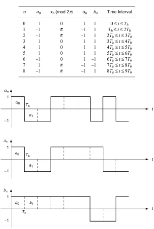
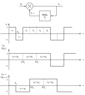
Fig. 2-9. An example of the equivalent I and Q data sequences represented as rectangular pulse streams. Redrawn from [1].
1
α
0
α
n
α
n
α π
Tb
1
−1
t
t an
a0
a1
Tb
1
−1
bn
b0 b1
Tb
1
−1
t xn (mod 2 )
n an bn Time Interval
0 1 2 3 4 5 6 7 8
0
0 0 0 0
π π
π π
1 −1 −1 1 1 1 −1 1 −1
1 −1 −1 1 1 1 1 −1 −1
1 1 1 1 1 1 −1 −1 1
0 ≤t≤Tb
Tb≤t≤ 2Tb
cn = (−1)na2n−1
dn = (−1)nb2n
(2.8 28)
To complete the analogy between MSK and sinusoidally pulse shaped OQPSK, we must examine the manner in which the equivalent I and Q data sequences needed in (2.8-28) are obtained from the input data sequence {αn}.
Without going into great mathematical detail, we can say that it can be shown that the sequences {a2n−1} and {b2n} are the odd/even split of a sequence,
{vn}, which is the differentially encoded version of{αn}, i.e.,vn =αnvn−1 (see
Fig. 2-10 for an illustrative example). Finally, the I-Q implementation of MSK as described by (2.8-26)–(2.8-28) is illustrated in Fig. 2-11. As anticipated, we observe that this figure resembles a transmitter for OQPSK except that here, the pulse shaping is half-sinusoidal (of symbol duration Ts = 2Tb) rather than
rectangular; in addition, we see that a differential encoder is applied to the input data sequence prior to splitting it into even and odd sequences, each at a rate 1/Ts. The interpretation of MSK as a special case of OQPSK with sinusoidal
pulse shaping along with trade-offs and comparisons between the two modula-tions is further discussed in Refs. 22 and 23.
Before concluding this section, we note that the alternative representation of MSK as in (2.8-22) can be also expressed in terms of the differentially encoded bits,vn. In particular,
Fornodd
sMSK(t) =
2Eb
Tb
vn−1+vn
2 cos 2π
fc+
1 4Tb
t
−
vn−1−vn
2 cos 2π
fc− 1
4Tb
t
,
nTb≤t≤(n+ 1)Tb (2.8 29a)
Forneven
sMSK(t) =
2Eb
Tb
vn−1+vn
2 cos 2π
fc+
1 4Tb
t
+
vn−1−vn
2 cos 2π
fc−
1 4Tb
t
,
νn
ν5
ν4
ν3
ν2
ν1
ν1
Fig. 2-10. An example of the equivalence between differentially encoded inputs bits and effective I and Q bits. Redrawn from [1].
n
α
νn −1
νn
Delay Tb
Tb 1
−1
t
ν2n
(b2n )
ν2n −1 (a2n −1)
ν 0 = b0 ν 2 = b2
ν 1 = a1
ν 3 = a3 ν 5 = a5
ν 4 = b4
2Tb
3Tb 5Tb
4Tb 1
−1
t
Tb
1
−1
t
Combining these two results we get
sMSK(t) =
2Eb
Tb
vn−1+vn
2
cos
2π
fc+
1 4Tb
t
+ (−1)n
vn−1−vn
2
cos
2π
fc− 1
4Tb
t
,
Differential Encoder
Delay Tb
Serial to Parallel Converter
s (t)
S (t) C (t)
k
α
k −1
ν
Qk
ν
Ik
ν
k
ν
cos 2πfct
2πfct sin
k
α MSK or SFSK
Frequency Modulator
s (t)
Fig. 2-11. CPM and equivalent I-Q implementations of MSK or SFSK.
Fig. 2-12. An I-Q receiver implementation of MSK.
∫
1
−1 1
−1
Data Combiner
Differential Decoder
b2n
n
ν α n
a2n −1
(2n +1)Tb
(2n −1)Tb
r (t)
C (t)
S (t) zc(t)
zs(t)
( )dt
∫
(2n +2)Tb2nTb