Joe Celko's Data and Databases: Concepts in Practice
by Joe Celko ISBN: 1558604324
Morgan Kaufmann Publishers © 1999, 382 pages
A "big picture" look at database design and programming for all levels of developers.
Table of Contents Colleague Comments
Back Cover
Synopsis by Dean Andrews
In this book, outspoken database magazine columnist Joe Celko waxes philosophic about fundamental concepts in database design and
development. He points out misconceptions and plain ol' mistakes commonly made while creating databases including mathematical calculation errors, inappropriate key field choices, date representation goofs and more. Celko also points out the quirks in SQL itself. A detailed table-of-contents will quickly route you to your area of interest.
Table of Contents
Joe Celko’s Data and Databases: Concepts in Practice - 4
Preface - 6
Chapter 1
-
The Nature of Data - 13Chapter 2
- Entities, Attributes, Values, and Relationships
- 23Chapter 3
-
Data Structures - 31Chapter 4
- Relational Tables
- 49Chapter 5
-
Access Structures - 69Chapter 6
- Numeric Data
- 84Chapter 7
-
Character String Data - 92Chapter 8
- Logic and Databases
- 104Chapter 9
-
Temporal Data - 123Chapter 10
- Textual Data
- 131Chapter 11
-
Exotic Data - 135Chapter 12
- Scales and Measurements
- 146Chapter 13
-
Missing Data - 151Chapter 15
- Check Digits
- 163Chapter 16
-
The Basic Relational Model - 178Chapter 17
- Keys
- 188Chapter 18
-
Different Relational Models - 202Chapter 19
- Basic Relational Operations
- 205Chapter 20
-
Transactions and Concurrency Control - 207Chapter 21
- Functional Dependencies
- 214Chapter 22
-
Normalization - 217Chapter 23
- Denormalization
- 238Chapter 24
-
Metadata - 252References - 258
Back Cover
Do you need an introductory book on data and databases? If the book is by Joe Celko, the answer is yes. Data & Databases: Concepts in Practice is the first introduction to relational database technology written especially for practicing IT professionals. If you work mostly outside the database world, this book will ground you in the concepts and overall framework you must master if your data-intensive projects are to be successful. If you’re already an experienced database programmer, administrator, analyst, or user, it will let you take a step back from your work and examine the founding principles on which you rely every day -- helping you work smarter, faster, and problem-free.
Whatever your field or level of expertise, Data & Databases offers you the depth and breadth of vision for which Celko is famous. No one knows the topic as well as he, and no one conveys this knowledge as clearly, as effectively -- or as engagingly. Filled with absorbing war stories and no-holds-barred commentary, this is a book you’ll pick up again and again, both for the information it holds and for the distinctive style that marks it as genuine Celko.
Features:
• Supports its extensive conceptual information with example code and other practical illustrations.
• Explains fundamental issues such as the nature of data and data modeling and moves to more specific technical questions such as scales, measurements, and encoding.
• Offers fresh, engaging approaches to basic and not-so-basic issues of database programming, including data entities, relationships and values, data structures, set operations, numeric data, character string data, logical data and operations, and missing data.
• Covers the conceptual foundations of modern RDBMS technology, making it an ideal choice for students.
Joe Celko is a noted consultant, lecturer, writer, and teacher, whose column in
Intelligent Enterprise has won several Reader’s Choice Awards. He is well known for his ten years of service on the ANSI SQL standards committee, his dependable help on the DBMS CompuServe Forum, and, of course, his war stories, which provide real-world insight into SQL programming.
Joe Celko’s Data and Databases: Concepts in
Practice
Joe Celko
Senior Editor: Diane D. Cerra
Director of Production and Manufacturing: Yonie Overton Production Editor: Cheri Palmer
Editorial Coordinator: Belinda Breyer
Cover and Text Design: Side by Side Studios Cover and Text Series Design: ThoughtHouse, Inc. Copyeditor: Ken DellaPenta
Proofreader: Jennifer McClain Composition: Nancy Logan Illustration: Cherie Plumlee Indexer: Ty Koontz
Printer: Courier Corporation
Designations used by companies to distinquish their products are often claimed as trademarks or registered trademarks. In all instances where Morgan Kaufmann Publishers is aware of a claim, the product names appear in initial capital or all capital letters. Readers, however, should contact the appropriate companies for more complete information regarding trademarks and registration.
Morgan Kaufmann Publishers Editorial and Sales Office 340 Pine Street, Sixth Floor San Francisco, CA 94104-3205 USA
Telephone: 415/392-2665 Facsimile: 415-982-2665 E-mail: [email protected] www: http://www.mkp.com
Order toll free: 800/745-7323
Printed in the United States of America
To my father, Joseph Celko Sr., and to my daughters, Takoga Stonerock and Amanda Pattarozzi
Preface
Overview
This book is a collection of ideas about the nature of data and databases. Some of the material has appeared in different forms in my regular columns in the computer trade and academic press, on CompuServe forum groups, on the Internet, and over beers at conferences for several years. Some of it is new to this volume.
This book is not a complete, formal text about any particular database theory and will not be too mathematical to read easily. Its purpose is to provide foundations and philosophy to the working programmer so that they can understand what they do for a living in greater depth. The topic of each chapter could be a book in itself and usually has been.
This book is supposed to make you think and give you things to think about. Hopefully, it succeeds.
Thanks to my magazine columns in DBMS, Database Programming & Design, Intelligent Enterprise, and other publications over the years, I have become the apologist for ANSI/ISO standard SQL. However, this is not an SQL book per se. It is more oriented toward the philosophy and foundations of data and databases than toward programming tips and techniques. However, I try to use the ANSI/ISO SQL-92 standard language for examples whenever possible, occasionally extending it when I have to invent a notation for some purpose.
If you need a book on the SQL-92 language, you should get a copy of Understanding the New SQL, by Jim Melton and Alan Simon (Melton and Simon 1993). Jim’s other book, Understanding SQL’s Stored Procedures (Melton 1998), covers the procedural language that was added to the SQL-92 standard in 1996.
If you want to get SQL tips and techniques, buy a copy of my other book, SQL for Smarties (Celko 1995), and then see if you learned to use them with a copy of SQL Puzzles & Answers (Celko 1997).
Organization of the Book
The book is organized into nested, numbered sections arranged by topic. If you have a problem and want to look up a possible solution now, you can go to the index or table of contents and thumb to the right section. Feel free to highlight the parts you need and to write notes in the margins.
Corrections and Future Editions
I will be glad to receive corrections, comments, and other suggestions for future editions of this book. Send your ideas to
Joe Celko
235 Carter Avenue Atlanta, GA 30317-3303
email: [email protected] website: www.celko.com
or contact me through the publisher. You could see your name in print!
Acknowledgments
I’d like to thank Diane Cerra of Morgan Kaufmann and the many people from CompuServe forum sessions and personal letters and emails. I’d also like to thank all the members of the ANSI X3H2 Database Standards Committee, past and present.
Chapter 1:
The Nature of Data
Where is the wisdom? Lost in the knowledge. Where is the knowledge? Lost in the information. —T. S. Eliot
Where is the information? Lost in the data. Where is the data?
Lost in the #@%&! database! — Joe Celko
Overview
So I am not the poet that T. S. Eliot is, but he probably never wrote a computer program in his life. However, I agree with his point about wisdom and information. And if he knew the distinction between data and information, I like to think that he would have agreed with mine.
I would like to define “data,” without becoming too formal yet, as facts that can be represented with measurements using scales or with formal symbol systems within the context of a formal model. The model is supposed to represent something called “the real world” in such a way that changes in the facts of “the real world” are reflected by changes in the database. I will start referring to “the real world” as “the reality” for a model from now on.
I will argue that the first databases were the precursors to written language that were found in the Middle East (see Jean 1992). Shepherds keeping community flocks needed a way to manipulate ownership of the animals, so that everyone knew who owned how many rams, ewes, lambs, and whatever else. Rather than branding the individual animals, as Americans did in the West, each member of the tribe had a set of baked clay tokens that represented ownership of one animal, but not of any animal in particular.
When you see the tokens, your first thought is that they are a primitive internal currency system. This is true in part, because the tokens could be traded for other goods and services. But their real function was as a record keeping system, not as a way to measure and store economic value. That is, the trade happened first, then the tokens were changed, and not vice versa.
The tokens had all the basic operations you would expect in a database. The tokens were updated when a lamb grew to become a ram or ewe, deleted when an animal was eaten or died, and new tokens were inserted when the new lambs were born in the spring.
One nice feature of this system is that the mapping from the model to the real world is one to one and could be done by a man who cannot count or read. He had to pass the flock through a gate and match one token to one animal; we would call this a “table scan” in SQL. He would hand the tokens over to someone with more math ability—the CPU for the tribe—who would update everyone’s set of tokens. The rules for this sort of updating can be fairly elaborate, based on dowry payments, oral traditions, familial relations, shares owned last year, and so on.
The tokens were stored in soft clay bottles that were pinched shut to ensure that they were not tampered with once accounts were settled; we would call that “record locking” in database management systems.
1.1 Data versus Information
Information is what you get when you distill data. A collection of raw facts does not help anyone to make a decision until it is reduced to a higher-level abstraction. My
sheepherders could count their tokens and get simple statistical summaries of their holdings (“Abdul owns 15 ewes, 2 rams, and 13 lambs”), which is immediately useful, but it is very low-level information.
If Abdul collected all his data and reduced it to information for several years, then he could move up one more conceptual level and make more abstract statements like, “In the years when the locusts come, the number of lambs born is less than the following two years,” which are of a different nature than a simple count. There is both a long time horizon into the past and an attempt to make predictions for the future. The information is qualitative and not just quantitative.
1.2 Information versus Wisdom
Wisdom does not come out of the database or out of the information in a mechanical fashion. It is the insight that a person has to make from information to handle totally new situations. I teach data and information processing; I don’t teach wisdom. However, I can say a few remarks about the improper use of data that comes from bad reasoning.
1.2.1 Innumeracy
Innumeracy is a term coined by John Allen Paulos in his 1990 best-seller of the same title. It refers to the inability to do simple mathematical reasoning to detect bad data, or bad reasoning. Having data in your database is not the same thing as knowing what to do with it. In an article in Computerworld, Roger L. Kay does a very nice job of giving
examples of this problem in the computer field (Kay 1994).
1.2.2 Bad Math
Bruce Henstell (1994) stated in the Los Angeles Times: “When running a mile, a 132 pound woman will burn between 90 to 95 calories but a 175 pound man will drop 125 calories. The reason seems to be evolution. In the dim pre-history, food was hard to come by and every calorie has to be conserved—particularly if a woman was to conceive and bear a child; a successful pregnancy requires about 80,000 calories. So women should keep exercising, but if they want to lose weight, calorie count is still the way to go.”
Calories are a measure of the energy produced by oxidizing food. In the case of a person, calorie consumption depends on the amount of oxygen they breathe and the body material available to be oxidized.
Let’s figure out how many calories per pound of human flesh the men and women in this article were burning: (95 calories/132 pounds) = .71 calories per pound of woman and (125 calories/175 pounds) = .71 calories per pound of man. Gee, there is no difference at all! Based on these figures, human flesh consumes calories at a constant rate when it exercises regardless of gender. This does not support the hypothesis that women have a harder time losing fat through exercise than men, but just the opposite. If anything, this shows that reporters cannot do simple math.
Another example is the work of Professor James P. Allen of Northridge University and Professor David Heer of USC. In late 1991, they independently found out that the 1990 census for Los Angeles was wrong. The census showed a rise in Black Hispanics in South Central Los Angeles from 17,000 in 1980 to almost 60,000 in 1990. But the total number of Black citizens in Los Angeles has been dropping for years as they move out to the suburbs (Stewart 1994).
Furthermore, the overwhelming source of the Latino population is Mexico and then Central America, which have almost no Black population. In short, the apparent growth of Black Hispanics did not match the known facts.
Professor Heer did it with just the data. The census questionnaire asked for race as White, Black, or Asian, but not Hispanic. Most Latinos would not answer the race question—Hispanic is the root word of “spic,” an ethnic slander word in Southern
California. He found that the Census Bureau program would assign ethnic groups when it was faced with missing data. The algorithm was to look at the makeup of the neighbors and assume that missing data was the same ethnicity.
If only they had NULLs to handle the missing data, they might have been saved.
Speaker’s Idea File (published by Ragan Publications, Chicago) lost my business when they sent me a sample issue of their newsletter that said, “On an average day,
approximately 140,000 people die in the United States.” Let’s work that out using 365.2422 days per year times 140,000 deaths for a total of 51,133,908 deaths per year. Since there are a little less than 300 million Americans as of the last census, we are looking at about 17% of the entire population dying every year—one person in every five or six. This seems a bit high. The actualfigure is about 250,000 deaths per year.
There have been a series of controversial reports and books using statistics as their basis. Tainted Truth: The Manipulation of Facts in America, by Cynthia Crossen, a reporter for the Wall Street Journal, is a study of how political pressure groups use “false facts” for their agenda (Crossen 1996). So there are reporters who care about
mathematics, after all!
Who Stole Feminism?, by Christina Hoff Sommers, points out that feminist authors were quoting a figure of 150,000 deaths per year from anorexia when the actual figure was no higher than 53. Some of the more prominent feminist writers who used this figure were Gloria Steinem (“In this country alone. . . about 150,000 females die of anorexia each year,” in Revolution from Within) and Naomi Wolf (“When confronted by such a vast number of emaciated bodies starved not by nature but by men, one must notice a certain resemblance [to the Nazi Holocaust],” in The Beauty Myth). The same false statistic also appears in Fasting Girls: The Emergence of Anorexia Nervosa as a Modern Disease, by Joan Brumberg, former director of Women’s Studies at Cornell, and hundreds of
newspapers that carried Ann Landers’s column. But the press never questioned this in spite of the figure being almost three times the number of dead in the entire 10 years of the Vietnam War (approximately 58,000) or in one year of auto accidents (approximately 48,000).
You might be tempted to compare this to the Super Bowl Sunday scare that went around in the early 1990s (the deliberate lie that more wives are beaten on Super Bowl Sunday than any other time). The original study only covered a very small portion of a select group—African Americans living in public housing in one particular part of one city. The author also later said that her report stated nothing of the kind, remarking that she had been trying to get the urban myth stopped for many months without success. She noted that the increase was considered “statistically insignificant” and could just as easily have been caused by bad weather that kept more people inside.
The broadcast and print media repeated it without even attempting to verify its accuracy, and even broadcasted public warning messages about it. But at least the Super Bowl scare was not obviously false on the face of it. And the press did do follow-up articles showing which groups created and knowingly spread a lie for political reasons.
1.2.3 Causation and Correlation
be present for an effect to happen—a car has to have gas to run. A sufficient cause will bring about the effect by itself—dropping a hammer on your foot will make you scream in pain, but so will having your hard drive crash. A contributory cause is one that helps the effect along, but would not be necessary or sufficient by itself to create the effect. There are also coincidences, where one thing happens at the same time as another, but without a causal relationship.
A correlation between two measurements, say, X and Y, is basically a formula that allows you to predict one measurement given the other, plus or minus some error range. For example, if I shot a cannon locked at a certain angle, based on the amount of gunpowder I used, I could expect to place the cannonball within a 5-foot radius of the target most of the time. Once in awhile, the cannonball will be dead on target; other times it could be several yards away.
The formula I use to make my prediction could be a linear equation or some other function. The strength of the prediction is called the coefficient of correlation and is denoted by the variable r where –1 = r = 1, in statistics. A coefficient of correlation of –1 is absolute negative correlation—when X happens, then Y never happens. A coefficient of correlation of +1 is absolute positive correlation—when X happens, then Y also happens. A zero coefficient of correlation means that X and Y happen independently of each other.
The confidence level is related to the coefficient of correlation, but it is expressed as a percentage. It says that x % of the time, the relationship you have would not happen by chance.
The study of secondhand smoke (or environmental tobacco smoke, ETS) by the EPA, which was released jointly with the Department of Health and Human Services, is a great example of how not to do a correlation study. First they gathered 30 individual studies and found that 24 of them would not support the premise that secondhand smoke is linked to lung cancer. Next, they combined 11 handpicked studies that used completely different methods into one sample—a technique known as metanalysis, or more informally called the apples and oranges fallacy. Still no link. It is worth mentioning that one of the rejected studies was recently sponsored by the National Cancer Institute— hardly a friend of the tobacco lobby—and it also showed no statistical significance.
The EPA then lowered the confidence level from 98% to 95%, and finally to 90%, where they got a relationship. No responsible clinical study has ever used less than 95% for its confidence level. Remember that a confidence level of 95% says that 5% of the time, this could just be a coincidence. A 90% confidence level doubles the chances of an error.
Alfred P. Wehner, president of Biomedical and Environmental Consultants Inc. in Richland, Washington, said, “Frankly, I was embarrassed as a scientist with what they came up with. The main problem was that statistical handling of the data.” Likewise, Yale University epidemiologist Alvan Feinstein, who is known for his work in experimental design, said in the Journal of Toxicological Pathologythat he heard a prominent leader in epidemiology admit, “Yes, it’s [EPA’s ETS work] rotten science, but it’s in a worthy cause. It will help us get rid of cigarettes and to become a smoke-free society.” So much for scientific truth versus a political agenda.
There are five ways two variables can be related to each other. The truth could be that X causes Y. You can estimate the temperature in degrees Fahrenheit from the chirp rate of a cricket: degrees = (chirps + 137.22)/3.777, with r = 0.9919 accuracy. However, nobody believes that crickets cause temperature changes. The truth could be that Y causes X, case two.
The third case is that X and Y interact with each other. Supply and demand curves are an example, where as one goes up, the other goes down (negative feedback in computer terms). A more horrible example is drug addiction, where the user requires larger and larger doses to get the desired effect (positive feedback in computer terms), as opposed to habituation, where the usage hits an upper level and stays there.
The fourth case is that any relationship is pure chance. Any two trends in the same direction will have some correlation, so it should not surprise you that once in awhile, two will match very closely.
The final case is where the two variables are effects of another variable that is outside the study. The most common unseen variables are changes in a common environment. For example, severe hay fever attacks go up when corn prices go down. They share a common element—good weather. Good weather means a bigger corn crop and hence lower prices, but it also means more ragweed and pollen and hence more hay fever attacks. Likewise, spouses who live pretty much the same lifestyle will tend to have the same medical problems from a common shared environment and set of habits.
1.2.4 Testing the Model against Reality
The March 1994 issue of Discovery magazine had a commentary column entitled “Counting on Dyscalculia” by John Allen Paulos. His particular topic was health statistics since those create a lot of “pop dread” when they get played in the media.
One of his examples in the article was a widely covered lawsuit in which a man alleged a causal connection between his wife’s frequent use of a cellular phone and her
subsequent brain cancer. Brain cancer is a rare disease that strikes approximately 7 out of 100,000 people per year. Given the large population of the United States, this is still about 17,500 new cases per year—a number that has held pretty steady for years.
There are an estimated 10 million cellular phone users in the United States. If there were a causal relationship, then there would be an increase in cases as cellular phone usage increased. On the other hand, if we found that there were less than 70 cases among cellular phone users we could use the same argument to “prove” that cellular phones prevent brain cancer.
Perhaps the best example of testing a hypothesis against the real world was the bet between the late Julian Simon and Paul Ehrlich (author of The Population Bomb and a whole raft of other doomsday books) in 1980. They took an imaginary $1,000 and let Ehrlich pick commodities. The bet was whether the real price would go up or down, depending on the state of the world, in the next 10 years. If the real price (i.e., adjusted for inflation) went down, then Simon would collect the adjusted real difference in current dollars; if the real costs went up, then Ehrlich would collect the difference adjusted to current dollars.
not adjusted for inflation, he would still have lost!
1.3 Models versus Reality
A model is not reality, but a reduced and simplified version of it. A model that was more complex than the thing it attempts to model would be less than useless. The term “the real world” means something a bit different than what you would intuitively think. Yes, physical reality is one “real world,” but this term also includes a database of information about the fictional worlds in Star Trek,the “what if” scenarios in a spreadsheet or discrete simulation program, and other abstractions that have no physical forms. The main characteristic of “the real world” is to provide an authority against which to check the validity of the database model.
A good model reflects the important parts of its reality and has predictive value. A model without predictive value is a formal game and not of interest to us.
The predictive value does not have to be absolutely accurate. Realistically, Chaos Theory shows us that a model cannot ever be 100% predictive for any system with enough structure to be interesting and has a feedback loop.
1.3.1 Errors in Models
Statisticians classify experimental errors as Type I and Type II. A Type I error is
accepting as false something that is true. A Type II error is accepting as true something that is false. These are very handy concepts for database people, too.
The classic Type I database error is the installation in concrete of bad data, accompanied by the inability or unwillingness of the system to correct the error in the face of the truth. My favorite example of this is a classic science fiction short story written as a series of letters between a book club member and the billing computer. The human has returned an unordered copy of Kidnapped by Robert Louis Stevenson and wants it credited to his account.
When he does not pay, the book club computer turns him over to the police computer, which promptly charges him with kidnapping Robert Louis Stevenson. When he objects, the police computer investigates, and the charge is amended to kidnapping and murder, since Robert Louis Stevenson is dead. At the end of the story, he gets his refund credit and letter of apology after his execution.
While exaggerated, the story hits all too close to home for anyone who has fought a false billing in a system that has no provision for clearing out false data.
The following example of a Type II error involves some speculation on my part. Several years ago a major credit card company began to offer cards in a new designer color with higher limits to their better customers. But if you wanted to keep your old card, you could have two accounts. Not such a bad option, since you could use one card for business and one for personal expenses.
They needed to create new account records in their database (file system?) for these new cards. The solution was obvious and simple: copy the existing data from the old account without the balances into the new account and add a field to flag the color of the card to get a unique identifier on the new accounts.
some were for the new card without any prior history, and some were for the new “two accounts” option.
One of the fields was the date of first membership. The company thinks that this date is very important since they use it in their advertising. They also think that if you do not use a card for a long period of time (one year), they should drop your membership. They have a program that looks at each account and mails out a form letter to these unused
accounts as it removes them from the database.
The brand new accounts were fine. The replacement accounts were fine. But the members who picked the “two card” option were a bit distressed. The only date that the system had to use as “date of last card usage” was the date that the original account was opened. This was almost always more than one year, since you needed a good credit history with the company to get offered the new card.
Before the shiny new cards had been printed and mailed out, the customers were getting drop letters on their new accounts. The switchboard in customer service looked like a Christmas tree. This is a Type II error—accepting as true the falsehood that the last usage date was the same as the acquisition date of the credit card.
1.3.2 Assumptions about Reality
The purpose of separating the formal model and the reality it models is to first
acknowledge that we cannot capture everything about reality, so we pick a subset of the reality and map it onto formal operations that we can handle.
This assumes that we can know our reality, fit it into a formal model, and appeal to it when the formal model fails or needs to be changed.
This is an article of faith. In the case of physical reality, you can be sure that there are no logical contradictions or the universe would not exist. However, that does not mean that you have full access to all the information in it. In a constructed reality, there might well be logical contradictions or vague information. Just look at any judicial system that has been subjected to careful analysis for examples of absurd, inconsistent behavior.
But as any mathematician knows, you have to start somewhere and with some set of primitive concepts to be able to build any model.
Chapter 2:
Entities, Attributes, Values, and
Relationships
Perfection is finally attained not when there is no longer anything to add but when there is no longer anything to take away.
—Antoine de Saint Exupery
Overview
What primitives should we use to build a database? The smaller the set of primitives, the better a mathematician feels. A smaller set of things to do is also better for an
they are very well defined for us.
Entities, attributes, values, and relationships are the components of a relational model. They are all represented as tables made of rows, which are made of columns in SQL and the relational model, but their semantics are very different. As an aside, when I teach an SQL class, I often have to stress that a table is made of rows, and not rows and columns; rows are made of columns. Many businesspeople who are learning the relational model think that it is a kind of spreadsheet, and this is not the case. A spreadsheet is made up of rows and columns, which have equal status and meaning in that family of tools. The cells of a spreadsheet can store data or programs; a table stores only data and constraints on the data. The spreadsheet is active, and the relational table is passive.
2.1 Entities
An entity can be a concrete object in its reality, such as a person or thing, or it can be a relationship among objects in its reality, such as a marriage, which can handled as if it were an object. It is not obvious that some information should always be modeled as an entity, an attribute, or a relationship. But at least in SQL you will have a table for each class of entity, and each row will represent one instance of that class.
2.1.1 Entities as Objects
Broadly speaking, objects are passive and are acted upon in the model. Their attributes are changed by processes outside of themselves. Properly speaking, each row in an object table should correspond to a “thing” in the database’s reality, but not always uniquely. It is more convenient to handle a bowl of rice as a single thing instead of giving a part number to each grain.
Clearly, people are unique objects in physical reality. But if the same physical person is modeled in a database that represents a company, they can have several roles. They can be an employee, a stockholder, or a customer.
But this can be broken down further. As an employee, they can hold particular positions that have different attributes and powers; the boss can fire the mail clerk, but the mail clerk cannot fire the boss. As a stockholder, they can hold different classes of stock, which have different attributes and powers. As a customer, they might get special discounts from being a customer-employee.
The question is, Should the database model the reality of a single person or model the roles they play? Most databases would model reality based on roles because they take actions based on roles rather than based on individuals. For example, they send
paychecks to employees and dividend checks to stockholders. For legal reasons, they do not want to send a single check that mixes both roles.
It might be nice to have a table of people with all their addresses in it, so that you would be able to do a change of address operation only once for the people with multiple roles. Lack of this table is a nuisance, but not a disaster. The worst you will do is create redundant work and perhaps get the database out of synch with the reality. The real problems can come when people with multiple roles have conflicting powers and actions within the database. This means that the model was wrong.
A relationship is a way of tying objects together to get new information that exists apart from the particular objects. The problem is that the relationship is often represented by a token of some sort in the reality.
A marriage is a relationship between two people in a particular legal system, and its token is the marriage license. A bearer bond is also a legal relationship where either party is a lawful individual (i.e., people, corporations, or other legal creations with such rights and powers).
If you burn a marriage license, you are still married; you have to burn your spouse instead (generally frowned upon) or divorce them. The divorce is the legal procedure to drop the marriage relationship. If you burn a bearer bond, you have destroyed the relationship. A marriage license is a token that identifies and names the relationship. A bearer bond is a token that contains or is itself the relationship.
You have serious problems when a table improperly models a relationship and its entities at the same time. We will discuss this problem in section 2.5.1.
2.2 Attributes
Attributes belong to entities and define them. Leibniz even went so far as to say that an entity is the sum of all its attributes. SQL agrees with this statement and models attributes as columns in the rows of tables that can assume values.
You should assume that you cannot ever show in a table all the attributes that an entity has in its reality. You simply want the important ones, where “important” is defined as those attributes needed by the model to do its work.
2.3 Values
A value belongs to an attribute. The particular value for a particular attribute is drawn from a domain or has a datatype. There are several schools of thought on domains, datatypes, and values, but the two major schools are the following:
1. Datatypes and domains are both sets of values in the database. They are both finite sets because all models are finite. The datatype differs by having operators in the hardware or software so the database user does not have to do all that work. A domain is built on a subset of a datatype, which inherits some or all of its operators from the original datatype and restrictions, but now the database can have user-defined operators on the domain.
2. A domain is a finite or infinite set of values with operators that exists in the database’s reality. A datatype is a subset of a domain supported by the computer the database resides on. The database approximates a domain with a subset of a datatype, which inherits some or all of its operators from the original datatype and other restrictions and operators given to it by the database designer.
Unfortunately, SQL-92 has a CREATEDOMAIN statement in its data declaration language (DDL) that refers to the approximation, so I will refer to database domains and reality domains.
definitions give a rule that determines if a value is in the domain or not. You have seen both of these approaches in elementary set theory in the list and rule notations for defining a set. For example, the finite set of positive even numbers less than 16 can be defined by either
A = {2, 4, 6, 8, 10, 12, 14}
or
B = {i : (MOD(i, 2) = 0) AND (i > 0) AND (i < 16)}
Defining the infinite set of all positive even numbers requires an ellipsis in the list notation, but the rule set notation simply drops restrictions, thus:
C = {2, 4, 6, 8, 10, 12, 14, . . .}
D = {i : MOD(i, 2) = 0}
While this distinction can be subtle, an intentional definition lets you move your model from one database to another much more easily. For example, if you have a machine that can handle integer datatypes that range up to (216) bits, then it is conceptually easy to move the database to a machine that can handle integer datatypes that range up to (232) bits because they are just two different approximations of the infinite domain of integers in the reality. In an extensional approach, they would be seen as two different datatypes without a reference to the reality.
For an abstract model of a DBMS, I accept a countably infinite set as complete if I can define it with a membership test algorithm that returns TRUE or FALSE in a finite amount of time for any element. For example, any integer can be tested for evenness in one step, so I have no trouble here.
But this breaks down when I have a test that takes an infinite amount of time, or where I cannot tell if something is an element of the set without generating all the previous elements. You can look up examples of these and other such misbehaved sets in a good math book (fractal sets, the (3 * n + 1) problem, generator functions without a closed form, and so forth).
The (3 * n + 1) problem is known as Ulam’s conjecture, Syracuse’s problem, Kakutani’s problem, and Hasse’s algorithm in the literature, and it can be shown by this procedure (see Lagarias 1985 for details).
FUNCTION ThreeN (i INTEGER IN, j INTEGER IN) RETURNS INTEGER; LANGUAGE SQL
BEGIN
DECLARE k INTEGER; SET k = 0;
WHILE k <= j LOOP
SET k = k + 1; IF i IN (1, 2, 4)
THEN ThreeN((i / 2), k) ELSE ThreeN((3 * i + 1), k); END LOOP;
RETURN 1 -- answer is True END WHILE;
We are trying to construct a subset of all the integers that test true according to the rules defined in this procedure. If the number is even, then divide it by two and repeat the procedure on that result. If the number is odd, then multiply it by three, add one, and repeat the procedure on that result. You keep repeating the procedure until it is reduced to one.
For example, if you start with 7, you get the sequence (7, 22, 11, 34, 17, 52, 26, 13, 40, 20, 10, 5, 16, 8, 4, 2, 1, . . .), and seven is a member of the set. Bet that took longer than you thought!
As a programming tip, observe that when a result becomes 1, 2, or 4, the procedure hangs in a loop, endlessly repeating that sequence. This could be a nonterminating program, if we are not careful!
An integer, i, is an element of the set K(j) when i fails to arrive at one on or before j iterations. For example, 7 is a member of K(17). By simply picking larger and larger values of j, you can set the range so high that any computer will break. If the j parameter is dropped completely, it is not known if there are numbers that never arrive at one. Or to put it another way, is this set really the set of all integers?
Well, nobody knows the last time I looked. I have to qualify that statement this way, because in my lifetime I have seen solutions to the four-color map theorem and Fermat’s Last theorem proven. But Gödel proved that there are always statements in logic that cannot be proven to be TRUE or FALSE, regardless of the amount of time or the number of axioms you are given.
2.4 Relationships
Relationships exist among entities. We have already talked about entities as relationships and how the line is not clear when you create a model.
2.5 ER Modeling
In 1976 Peter Chen invented entity-relationship (ER) modeling as a database design technique. The original diagrams used a box for an entity, a diamond for a relationship, and lines to connect them. The simplicity of the diagrams used in this method have made it the most popular database design technique in use today. The original method was very minimal, so other people have added other details and symbols to the basic diagram.
There are several problems with ER modeling:
I feel that people should spend more time actually designing data elements, as you can see from the number of chapters in this book devoted to data.
2. Although there can be more than one normalized schema from a single set of constraints, entities, and relationships, ER tools generate only one diagram. Once you have begun a diagram, you are committed to one schema design.
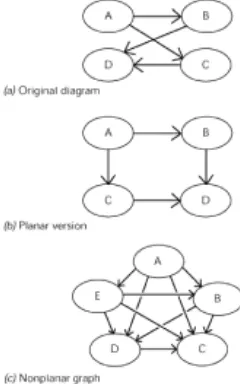
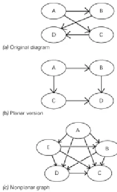
3. The diagram generated by ER tools tends to be a planar graph. That means that there are no crossed lines required to connect the boxes and lines. The fact that a graph has crossed lines does not make it nonplanar; it might be rearranged to avoid the crossed lines without changes to the connections (see Fig. 2.1).
Fig. 2.1
A planar graph can also be subject to another graph theory result called the “four-color map theorem,” which says that you only need four “four-colors to “four-color a planar map so that no two regions with a common border have the same color.
4. ER diagrams cannot express certain constraints or relationships. For example, in the versions that use only straight lines between entities for relationships, you cannot easily express an n-ary relationship (n > 2).
Furthermore, you cannot show constraint among the attributes within a table. For example, you cannot show the rule that “An employee must be at least 18 years of age” with a constraint of the form CHECK ((hiredate - birthdate) >= INTERVAL 18 YEARS).
As an example of the possibility of different schemas for the same problem, consider a database of horse racing information. Horses are clearly physical objects, and we need information about them if we are going to calculate a betting system. This modeling decision could lead to a table that looks like this:
CREATE TABLE Horses
track CHAR(30) NOT NULL,
race INTEGER NOT NULL CHECK (race > 0), racedate DATE NOT NULL,
position INTEGER NOT NULL CHECK (position > 0), finish CHAR(10) NOT NULL
CHECK (finish IN ('win', 'place', 'show', 'ran', 'scratch')), PRIMARY KEY (horsename, track, race, racedate));
The track column is the name of the track where the race was held, racedate is when it was held, race is the number of each race, position is the starting position of the horse, and finish is how well the animal did in the race. Finish is an attribute of the entity “horses” in this model. If you do not bet on horse races (“play the ponies”), “win” means first place; “place” is first or second place; “show” is first, second, or third place; “ran” is having been in the race, but not in first, second, or third place; and “scratch” means the horse was removed from the race in which it was scheduled to run. In this model, the finish attribute should have the highest value obtained by the horse in each row of the table.
Now look at the same reality from the viewpoint of the bookie who has to pay out and collect wagers. The most important thing in his model is the outcome of races, and detailed information on individual horses is of little interest. He might model the same reality with a table like this:
CREATE TABLE Races
(track CHAR(30) NOT NULL, racedate DATE NOT NULL,
race INTEGER NOT NULL CHECK (race > 0),
win CHAR(30) NOT NULL REFERENCES Horses(horsename), place CHAR(30) NOT NULL REFERENCES Horses(horsename), show CHAR(30) NOT NULL REFERENCES Horses(horsename), PRIMARY KEY (track, date, race));
The columns have the same meaning as they did in the Horses table, but now there are three columns with the names of the horse that won, placed, or showed for that race (“finished in the money”). Horses are values of attributes of the entity “races” in this model.
2.5.1 Mixed Models
We defined a mixed model as one in which a table improperly models both a relationship and its entities in the same column(s). When a table has a mixed model, you probably have serious problems. For example, consider the common adjacency list representation of an organizational chart:
CREATE TABLE Personnel
(emp_name CHAR(20) NOT NULL PRIMARY KEY,
boss_name CHAR(20) REFERENCES Personnel(emp_name),
dept_no CHAR(10) NOT NULL REFERENCES departments(dept_no), salary DECIMAL (10,2) NOT NULL,
. . . );
What is wrong with this table? First of all, this table is not normalized. Consider what happens when a middle manager named 'JerryRivers' decides that he needs to change his name to 'GeraldoRiviera' to get minority employment preferences. This change will have to be done once in the emp_name column and n times in the
boss_name column of each of his immediate subordinates. One of the defining
characteristics of a normalized database is that one fact appears in one place, one time, and one way in the database.
Next, when you see 'Jerry Rivers' in the emp_name column, it is a value for the name attribute of a Personnel entity. When you see 'Jerry Rivers' in the boss_name column, it is a relationship in the company hierarchy. In graph theory, you would say that this table has information on both the nodes and the edges of the tree structure in it.
There should be a separate table for the employees (nodes), which contains only
employee data, and another table for the organizational chart (edges), which contains only the organizational relationships among the personnel.
2.5 ER Modeling
In 1976 Peter Chen invented entity-relationship (ER) modeling as a database design technique. The original diagrams used a box for an entity, a diamond for a relationship, and lines to connect them. The simplicity of the diagrams used in this method have made it the most popular database design technique in use today. The original method was very minimal, so other people have added other details and symbols to the basic diagram.
There are several problems with ER modeling:
1. ER does not spend much time on attributes. The names of the columns in a table are usually just shown inside the entity box, without datatypes. Some products will indicate which column(s) are the primary keys of the table. Even fewer will use another notation on the column names to show the foreign keys.
I feel that people should spend more time actually designing data elements, as you can see from the number of chapters in this book devoted to data.
2. Although there can be more than one normalized schema from a single set of constraints, entities, and relationships, ER tools generate only one diagram. Once you have begun a diagram, you are committed to one schema design.
Fig. 2.1
A planar graph can also be subject to another graph theory result called the “four-color map theorem,” which says that you only need four “four-colors to “four-color a planar map so that no two regions with a common border have the same color.
4. ER diagrams cannot express certain constraints or relationships. For example, in the versions that use only straight lines between entities for relationships, you cannot easily express an n-ary relationship (n > 2).
Furthermore, you cannot show constraint among the attributes within a table. For example, you cannot show the rule that “An employee must be at least 18 years of age” with a constraint of the form CHECK((hiredate-birthdate)>=INTERVAL 18YEARS).
As an example of the possibility of different schemas for the same problem, consider a database of horse racing information. Horses are clearly physical objects, and we need information about them if we are going to calculate a betting system. This modeling decision could lead to a table that looks like this:
CREATE TABLE Horses
(horsename CHAR(30) NOT NULL, track CHAR(30) NOT NULL,
race INTEGER NOT NULL CHECK (race > 0), racedate DATE NOT NULL,
position INTEGER NOT NULL CHECK (position > 0), finish CHAR(10) NOT NULL
CHECK (finish IN ('win', 'place', 'show', 'ran', 'scratch')), PRIMARY KEY (horsename, track, race, racedate));
having been in the race, but not in first, second, or third place; and “scratch” means the horse was removed from the race in which it was scheduled to run. In this model, the finish attribute should have the highest value obtained by the horse in each row of the table.
Now look at the same reality from the viewpoint of the bookie who has to pay out and collect wagers. The most important thing in his model is the outcome of races, and detailed information on individual horses is of little interest. He might model the same reality with a table like this:
CREATE TABLE Races
(track CHAR(30) NOT NULL, racedate DATE NOT NULL,
race INTEGER NOT NULL CHECK (race > 0),
win CHAR(30) NOT NULL REFERENCES Horses(horsename), place CHAR(30) NOT NULL REFERENCES Horses(horsename), show CHAR(30) NOT NULL REFERENCES Horses(horsename), PRIMARY KEY (track, date, race));
The columns have the same meaning as they did in the Horses table, but now there are three columns with the names of the horse that won, placed, or showed for that race (“finished in the money”). Horses are values of attributes of the entity “races” in this model.
2.5.1 Mixed Models
We defined a mixed model as one in which a table improperly models both a relationship and its entities in the same column(s). When a table has a mixed model, you probably have serious problems. For example, consider the common adjacency list representation of an organizational chart:
CREATE TABLE Personnel
(emp_name CHAR(20) NOT NULL PRIMARY KEY,
boss_name CHAR(20) REFERENCES Personnel(emp_name),
dept_no CHAR(10) NOT NULL REFERENCES departments(dept_no), salary DECIMAL (10,2) NOT NULL,
. . . );
in which the column boss_name is the emp_name of the boss of this employee in the company hierarchy. This column has to allow a NULL because the hierarchy eventually leads to the head of the company, and he or she has no boss.
What is wrong with this table? First of all, this table is not normalized. Consider what happens when a middle manager named 'JerryRivers' decides that he needs to change his name to 'GeraldoRiviera' to get minority employment preferences. This change will have to be done once in the emp_name column and n times in the
boss_name column of each of his immediate subordinates. One of the defining
characteristics of a normalized database is that one fact appears in one place, one time, and one way in the database.
There should be a separate table for the employees (nodes), which contains only
employee data, and another table for the organizational chart (edges), which contains only the organizational relationships among the personnel.
2.6 Semantic Methods
Another approach to database design that was invented in the 1970s is based on semantics instead of graphs. There are several different versions of this basic approach, such as NIAM (Natural-language Information Analysis Method), BRM (Binary
Relationship Modeling), ORM (Object-Role Modeling), and FORM (Formal Object-Role Modeling). The main proponent of ORM is Terry Halpin, and I strongly recommend getting his book (Halpin 1995) for details of the method. What I do not recommend is using the diagrams in his method. In addition to diagrams, his method includes the use of simplified English sentences to express relationships. These formal sentences can then be processed and used to generate several schemas in a mechanical way.
Most of the sentences are structured as subject-verb-object, but the important thing is that the objects are assigned a role in the sentence. For example, the fact that “Joe Celko wrote Data and Databases for Morgan Kaufmann Publishers” can be amended to read “AUTHOR: Joe Celko wrote BOOK: ‘Data and Databases’ for PUBLISHER: Morgan Kaufmann,” which gives us the higher level, more abstract sentence that “Authors write books for publishers” as a final result, with the implication that there are many authors, books, and publishers involved. Broadly speaking, objects and entities become the subjects and objects of the sentences, relationships become verbs, and the constraints become prepositional phrases.
A major advantage of the semantic methods is that a client can check the simple
sentences for validity easily. An ER diagram, on the other hand, is not easily checked. One diagram looks as valid as another, and it is hard for a user to focus on one fact in the diagram.
Chapter 3:
Data Structures
Overview
Data structures hold data without regard to what the data is. The difference between a physical and an abstract model of a data structure is important, but often gets blurred when discussing them.
Each data structure has certain properties and operations that can be done on it, regardless of what is stored in it. Here are the basics, with informal definitions.
Data structures are important because they are the basis for many of the implementation details of real databases, for data modeling, and for relational operations, since tables are multisets.
3.1 Sets
use the term “empty set.”
The expression “same kind of thing” is a bit vague, but it is important. In a database, the rows of a table have to be instances of the same entity; that is, a Personnel table is made up of rows that represent individual employees. However, a grouped table built from the Personnel table, say, by grouping of departments, is not the same kind of element. In the grouped table, the rows are aggregates and not individuals. Departmental data is a different level of abstraction and cannot be mixed with individual data.
The basic set operations are the following:
• Membership: This operation says how elements are related to a set. An element either is or is not a member of a particular set. The symbol is ∈.
• Containment: One set A contains another set B if all the elements of B are also elements of A. B is called a subset of A. This includes the case where A and B are the same set, but if there are elements of A that are not in B, then the relationship is called proper containment. The symbol is ⊂; if you need to show “contains or equal to,” a horizontal bar can be placed under the symbol (⊆).
It is important to note that the empty set is not a proper subset of every set. If A is a subset of B, the containment is proper if and only if there exists an element b in B such that b is not in A. Since every set contains itself, the empty set is a subset of the empty set. But this is not proper containment, so the empty set is not a proper subset of every set.
• Union: The union of two sets is a single new set that contains all the elements in both sets. The symbol is ∪. The formal mathematical definition is
∀ x: x ∈ A ∨ x ∈ B ⇒ x ∈ (A ∪ B)
• Intersection: The intersection of two sets is a single new set that contains all the elements common to both sets. The symbol is ∩. The formal mathematical definition is
∀ x: x ∈ A ∧x ∈ B ⇒ x ∈ A ∩ B
• Difference: The difference of two sets A and B is a single new set that contains elements from A that are not in B. The symbol is a minus sign.
∀ x: x ∈ A ∧ ¬ (x ∈) B ⇒ x ∈ (A – B)
• Partition: The partition of a set A divides the set into subsets, A1, A2, . . . , An, such that
∪ A [i] = A ∧ ∩ A [i] = Ø
A multiset (also called a bag) is a collection of elements of the same type with duplicates of the elements in it. There is no ordering of the elements in a multiset, and we still have the empty set. Multisets have the same operations as sets, but with extensions to allow for handling the duplicates.
Multisets are the basis for SQL, while sets are the basis for Dr. Codd’s relational model.
The basic multiset operations are derived from set operations, but have extensions to handle duplicates:
• Membership: An element either is or is not a member of a particular set. The symbol is ∈. In addition to a value, an element also has a degree of duplication, which tells you the number of times it appears in the multiset.
Everyone agrees that the degree of duplication of an element can be greater than zero. However, there is some debate as to whether the degree of duplication can be zero, to show that an element is not a member of a multiset. Nobody has proposed using a negative degree of duplication, but I do not know if there are any reasons not to do so, other than the fact that it does not make any intuitive sense.
For the rest of this discussion, let me introduce a notation for finding the degree of duplication of an element in a set:
dod(<multiset>, <element>) = <integer value>
• Reduction: This operation removes redundant duplicates from the multiset and converts it into a set. In SQL, this is the effect of using a SELECT DISTINCT clause.
For the rest of this discussion, let me introduce a notation for the reduction of a set:
red(<multiset>)
•
Containment: One multiset A contains another multiset B if
1.red(A) ⊂ red(B)
2.∀ x ∈ B: dod(A, x) = dod(B, x)
This definition includes the case where A and B are the same multiset, but if there are elements of A that are not in B, then the relationship is called proper containment.
• Union: The union of two multisets is a single new multiset that contains all the elements in both multisets. A more formal definition is
∀ x: x ∈ A ∨ x ∈ B ⇒ x ∈ A ∪ B
∧
The degree of duplication in the union is the sum of the degree of duplication from both tables.
• Intersection: The intersection of two multisets is a single new multiset that contains all the elements common to both multisets.
∀ x: x ∈ A ∧ x ∈ B ⇒ x ∈ A ∩ B
∧
dod(A ∩ B, x) = ABS (dod(A, x) – dod(B B, x))
The degree of duplication in the intersection is based on the idea that you match pairs from each set in the intersection.
• Difference: The difference of two multisets A and B is a single new multiset that contains elements from A that are not in B after pairs are matched from the two multisets. More formally:
∀ x: x ∈ A ∧ ¬ (x ∈) B ⇒ x ∈ (A – B)
∧ dod((A – B), x) = (dod(A, x) – dod(B, x))
• Partition: The partition of a multiset A divides it into a collection of multisets, A1, A2, . . . , An, such that their multiset union is the original set and their multiset intersection is empty.
Because sets are so important in the relational model, we will return to them in Chapter 4
and go into more details.
3.3 Simple Sequential Files
Simple files are a linear sequence of identically structured records. There is a unique first record in the file. All the records have a unique successor except the unique last record. Records with identical content are differentiated by their position in the file. All processing is done with the current record.
In short, a simple sequential file is a multiset with an ordering added. In a computer system, these data structures are punch cards or magnetic tape files; in SQL this is the basis for CURSORs. The basic operations are the following:
• Open the file: This makes the data available. In some systems, it also positions a write head on the first record of the file. In others, such as CURSORs in SQL, the read-write head is positioned just before the first record of the file. This makes a difference in the logic for processing the file.
•
Fetch a record: This changes the current record and comes in several different flavors:
1.Fetch next: The successor of the current record becomes the new current record.
3.Fetch last: The last record becomes the new current record.
4.Fetch previous: The predecessor of the current record becomes the new current record.
5.Fetch absolute: The nth record becomes the new current record.
6.Fetch relative: The record n positions from the current record becomes the new current record.
There is some debate as to how to handle a fetch absolute or a fetch relative command that would position the read-write head before the first record or after the last record. One argument is that the current record should become the first or last record, respectively; another opinion is that an error condition should be raised.
In many older simple file systems and CURSOR implementations, only fetch next is available. The reason was obvious with punch card systems; you cannot “rewind” a punch card reader like a magnetic tape drive. The reason that early CURSOR
implementations had only fetch next is not so obvious, but had to do with the disposal of records as they were fetched to save disk storage space.
•
Close the file: This removes the file from the system.
• Insert a record: The new record becomes the current record, and the former current record becomes its successor.
• Update a record: Values within the current record are changed. The read-write does not change position.
• Delete a record:This removes a record from the file. The successor of the current record becomes the current record. If the current record was the last record of the file, the read-write head is positioned just past the end of the file.
3.4 Lists
A list is a sequence of elements, each of which can be either a scalar value called an atom or another list; the definition is recursive. The way that a list is usually displayed is as a comma-separated list within parentheses, as for example, ((Smith, John), (Jones, Ed)).
A list has only a few basic operations from which all other functions are constructed. The head() function returns the first element of a list, and the tail() function returns the rest of it. A constructor function builds a new list from a pair of lists, one for the head and one for the tail of the new list.
Lists are important in their own right, and the LISP programming language is the most common way to manipulate lists. However, we are interested in lists in databases because they can represent complex structures in a fast and compact form and are the basis for many indexing methods.
List programming languages also teach people to think recursively, since that is usually the best way to write even simple list procedures. As an example of a list function, consider Member(), which determines if a particular atom is in a list. It looks like this in pseudocode:
BOOLEAN PROCEDURE Member (a ATOM IN, l LIST IN) IF l IS ATOMIC
THEN RETURN (a = l) ELSE IF member(a, hd(l)) THEN RETURN TRUE
ELSE RETURN member(a, tl(l));
The predicate <list> IS ATOMIC returns TRUE if the list expression is an atom.
3.5 Arrays
Arrays are collections of elements accessed by using indexes. This terminology is unfortunate because the “index” of an array is a simple integer list that locates a value within the array, and not the index used on a file to speed up access. Another term taken from mathematics for “index” is “subscript,” and that term should be favored to avoid confusion.
Arrays appear in most procedural languages and are usually represented as a subscript list after the name of the array. They are usually implemented as contiguous storage locations in host languages, but linked lists can also be used. The elements of an array can be records or scalars. This is useful in a database because it gives us a structure in the host language into which we can put rows from a query and access them in a simple fashion.
3.6 Graphs
Graphs are made up of nodes connected by edges. They are the most general abstract data structure and have many different types. We do not need any of the more
complicated types of graphs in a database and can simply define an edge as a relationship between two nodes. The relationship is usually thought of in terms of a traversal from one node to another along an edge.
The two types of graphs that are useful to us are directed and undirected graphs. An edge in a directed graph can be traversed in only one direction; an edge in an undirected graph can be traversed in both directions. If I were to use a graph to represent the traffic patterns in a town, the one-way streets would be directed edges and the two-way streets would be undirected edges. However, a graph is never shown with both types of edges— instead, an undirected graph can be simulated in a directed graph by having all edges of the form (a,b) and (b,a) in the graph.
database, so we can model all of those things, too.
3.7 Trees
A tree is a special case of a graph. There are several equivalent definitions, but the most useful ones are the following:
• A tree is a graph with no cycles. The reason that this definition is useful to a database user is that circular references can cause a lot of problems within a database.
• A tree is made up of a node, called a parent, that points to zero or more other nodes, its children, or to another tree. This definition is recursive and therefore very compact, but another advantage is that this definition leads to a nested-sets model of
hierarchies.
Trees are the basis for indexing methods used in databases. The important operations on a tree are locating subtrees and finding paths when we are using them as an index. Searching is made easier by having rules to insert values into the tree. We will discuss this when we get to indexes.
Relational Philosopher
The creator of the relational model talks about his never-ending crusade.
Interviewing Dr. Edgar F. Codd about databases is a bit like interviewing Einstein about nuclear physics. Only no one has ever called the irascible Codd a saint. In place of Einstein’s publications on the theory of relativity, you have Codd’s ground-breaking 1970 paper on relational theory, which proposed a rigorous model for database management that offered the beguiling simplicity of the rows and columns of tables. But there was more to it than that. Codd’s work was firmly grounded in the mathematical theory of relations of arbitrary degree and the predicate logic first formulated by the ancient Greeks. Moreover, it was a complete package that handled mapping the real world to data structures as well as manipulating that data—that is, it included a specification for a normal form for database relations and the concept of a universal data sublanguage.
Almost as important to its success, Codd’s relational theory had Codd backing it. The former World War II Royal Air Force pilot made sure word got out from his IBM research lab to the world at large. In those early years he had to struggle against the political forces aligned behind IBM’s strategic database product, IMS, and came to work each day “wondering who was going to stab me in the back next.” Codd parried often and well, although observers say some of the blows Codd returned over the years were imagined or had even been struck for Codd’s own relational cause.
Codd won the great database debate and, with it, such laurels as the 1981 ACM (Association for Computing Machinery) Turing Award “for fundamental and continuing contributions to the theory and practice of database management systems.”
advocacy first let the genie out of the bottle. In place of Einstein’s political activism on behalf of peaceful uses of nuclear energy, Codd has aggressively campaigned to make sure “relational” is more than an advertising buzzword. Many a careless user of the word (and even some rather careful experts in the field) found themselves on the end of a scathing “Coddgram” for what Codd deemed their public misstatements. Some say his ComputerWorld articles of 1985 brought two major nonrelational database vendors to the verge of bankruptcy and then takeover.
Whereas Einstein’s work lead [sic] to the nuclear age, Codd’s work has lead [sic] to what might be called the relational age. Yet Codd is not resting or turning to new pursuits. He says his goal of protecting users of large databases from knowing how data is actually organized in the machine has been realized only in part. He says errors in the implementation of DBMS engines and the dominant data sublanguage, SQL, jeopardize data integrity and make it too hard to frame a very complex query and get back a usable answer.
Codd’s new book, The Relational Model for Database Management: Version 2, defines just how far he thinks we still have to go. It is highly recommended reading.
Whereas Code loves to elucidate the practical benefits of relational theory, things get dicey when talk ventures onto nonrelational grounds.
Einstein resisted new research done on quantum theory. Codd, in turn, resists nonrelational rumblings from the research community and DBMS vendors. Codd does not think much of work that extends the relational model (or skirts it) in order to deal more efficiently with data that doesn’t look like the text and numeric data of the SUPPLIER-PARTS-SUPPLY example popularized by Codd. His new book dismisses practically all database research of the last ten years in a brief chapter.
For Einstein, the practical predictive value of quantum theory never overcame his fundamental objection to it: “God doesn’t play dice with the universe.” Codd says his objection to the new directions in database research has no such element of the theological. The real problem, he says, is that the new work lacks a satisfactory theoretical foundation. Worse, he says, it violates the principals [sic] laid down in the theoretical foundations of the relational model.
If relational systems can’t deal effectively with the complex data found in
applications like CAD, CASE, and office automation, Codd says, it is because their implementation of the relational model is lacking, not their underlying theory. The point may be moot, however: Users and vendors are succumbing to the heady performance improvements offered by nonrelational (or imperfectly relational) alternatives.
What follows is an edited transcript of DBMS Editor in Chief Kevin Strehlo’s recent discussion with Dr. Codd.
DBMS: What got you started down the road toward those first papers on relational theory?
supported the existential quantifier. He said, “Well I get some funny questions, but