| Komputasi | Suatu Permulaan

(1)

Data

Structures

(2)

Author

The NetBeans IDE 5.5 runs on operating systems that support the Java VM. Below is a list of platforms:

• Microsoft Windows XP Professional SP2 or newer

• Mac OS X 10.4.5 or newer

• Red Hat Fedora Core 3

• Solaris™ 10 Operating System Update 1 (SPARC® and x86/x64 Platform Edition)

NetBeans Enterprise Pack is also known to run on the following platforms:

• Microsoft Windows 2000 Professional SP4

• Solaris™ 8 OS (SPARC and x86/x64 Platform Edition) and Solaris 9 OS (SPARC and x86/x64 Platform Edition)

• Various other Linux distributions Minimum Hardware Configuration

Note: The NetBeans IDE's minimum screen resolution is 1024x768 pixels.

• Microsoft Windows operating systems:

• Processor: 500 MHz Intel Pentium III workstation or

• Processor: UltraSPARC II 450 MHz

• Memory: 512 MB

• Disk space: 450 MB of free disk space

• Solaris OS (x86/x64 Platform Edition):

• Processor: AMD Opteron 100 Series 1.8 GHz

• Macintosh OS X operating system:

• Processor: PowerPC G4

Recommended Hardware Configuration

• Microsoft Windows operating systems:

• Processor: 1.4 GHz Intel Pentium III workstation or equivalent

• Memory: 1 GB

• Disk space: 1 GB of free disk space

• Linux operating system:

• Processor: 1.4 GHz Intel Pentium III or equivalent

• Solaris™ OS (SPARC®):

• Processor: UltraSPARC IIIi 1 GHz

(3)

• Solaris™ OS (x86/x64 platform edition):

• Processor: AMD Opteron 100 Series 1.8 GHz

• Macintosh OS X operating system:

• Processor: PowerPC G5

•

• Required Software

NetBeans Enterprise Pack 5.5 Early Access runs on the Java 2 Platform Standard Edition Development Kit 5.0 Update 1 or higher (JDK 5.0, version 1.5.0_01 or higher), which consists of the Java Runtime Environment plus developer tools for compiling, debugging, and running applications written in the Java language. Sun Java System Application Server Platform Edition 9 has been tested with JDK 5.0 update 6.

•

• For Solaris, Windows, and Linux, you can download the JDK for your platform from http://java.sun.com/j2se/1.5.0/download.html

(4)

1 Basic Concepts and Notations

1.1 Objectives

At the end of the lesson, the student should be able to:

• Explain the process of problem solving

• Define data type, abstract data type and data structure

• Identify the properties of an algorithm

• Differentiate the two addressing methods - computed addressing and link addressing

• Use the basic mathematical functions to analyze algorithms

• Measure complexity of algorithms by expressing the efficiency in terms of time complexity and big-O notation

1.2 Introduction

In creating a solution in the problem solving process, there is a need for representing higher level data from basic information and structures available at the machine level. There is also a need for synthesis of the algorithms from basic operations available at the machine level to manipulate higher-level representations. These two play an important role in obtaining the desired result. Data structures are needed for data representation while algorithms are needed to operate on data to produce correct output.

In this lesson we will discuss the basic concepts behind the problem-solving process, data types, abstract data types, algorithm and its properties, the addressing methods, useful mathematical functions and complexity of algorithms.

1.3 Problem Solving Process

Programming is a problem-solving process, i.e., the problem is identified, the data to manipulate and work on is distinguished and the expected result is determined. It is implemented in a machine known as a computer and the operations provided by the machine is used to solve the given problem. The problem solving process could be viewed in terms of domains – problem, machine and solution.

Problem domain includes the input or the raw data to process, and the output or the processed data. For instance, in sorting a set of numbers, the raw data is set of numbers in the original order and the processed data is the sorted numbers.

(10)

medium – bits, bytes, words, etc – consists of serially arranged bits that are addressable as a unit. The processing units allow us to perform basic operations that include arithmetic, comparison and so on.

Solution domain, on the other hand, links the problem and machine domains. It is at the solution domain where structuring of higher level data structures and synthesis of algorithms are of concern.

1.4 Data Type, Abstract Data Type and Data

Structure

Data type refers to the to the kind of data that variables can assume, hold or take on in a programming language and for which operations are automatically provided. In Java, the primitive data types are:

Keyword Description

boolean A boolean value (true or false)

Abstract Data Type (ADT), on the other hand, is a mathematical model with a collection of operations defined on the model. It specifies the type of data stored. It specifies what its operations do but not how it is done. In Java, ADT can be expressed with an interface, which contains just a list methods. For example, the following is an interface of the ADT stack, which we will cover in detail in Chapter 2:

public interface Stack{

public int size(); /* returns the size of the stack */ public boolean isEmpty(); /* checks if empty */

public Object top() throws StackException; public Object pop() throws StackException;

public void push(Object item) throws StackException; }

Data structure is the implementation of ADT in terms of the data types or other data structures. A data structure is modeled in Java by a class. Classes specify how

operations are performed. In Java, to implement an ADT as a data structure, an interface is implemented by a class.

(11)

understand and use.

1.5 Algorithm

Algorithm is a finite set of instructions which, if followed, will accomplish a task. It has five important properties: finiteness, definiteness, input, output and effectiveness.

Finiteness means an algorithm must terminate after a finite number of steps.

Definiteness is ensured if every step of an algorithm is precisely defined. For example, "divide by a number x" is not sufficient. The number x must be define precisely, say a positive integer. Input is the domain of the algorithm which could be zero or more quantities. Output is the set of one or more resulting quantities which is also called the range of the algorithm. Effectiveness is ensured if all the operations in the algorithm are sufficiently basic that they can, in principle, be done exactly and in finite time by a person using paper and pen.

Consider the following example:

public class Minimum {

public static void main(String[] args) {

int a[] = { 23, 45, 71, 12, 87, 66, 20, 33, 15, 69 }; int min = a[0];

for (int i = 1; i < a.length; i++) { if (a[i] < min) min = a[i]; }

System.out.println("The minimum value is: " + min);

}

The Java code above returns the minimum value from an array of integers. There is no user input since the data from where to get the minimum is already in the program. That is, for the input and output properties. Each step in the program is precisely defined. Hence, it is definite. The declaration, the for loop and the statement to output will all take a finite time to execute. Thus, the finiteness property is satisfied. And when run, it returns the minimum among the values in the array so it is said to be effective.

All the properties of an algorithm must be ensured in writing an algorithm.

1.6 Addressing Methods

In creating a data structure, it is important to determine how to access the data items. It is determined by the addressing method used. There are two types of addressing methods in general – computed and link addressing methods.

1.6.1 Computed Addressing Method

(12)

int x[] = new int[10];

A data item can be accessed directly by knowing the index on where it is stored.

1.6.2 Link Addressing Method

This addressing method provides the mechanism for manipulating dynamic structures where the size and shape are not known beforehand or if the size and shape changes at runtime. Central to this method is the concept of a node containing at least two fields: INFO and LINK.

Figure 1.1 Node Structure

In Java,

class Node{

Object info; Node link;

Node(){ }

Node(Object o, Node l){ info = o;

link = l; }

}

1.6.2.1 Linked Allocation: The Memory Pool

The memory pool is the source of the nodes from which linked structures are built. It is also known as the list of available space (or nodes) or simply the avail list:

(13)

The following is the Java class for AvailList:

class AvailList { Node head;

AvailList(){

head = null; }

AvailList(Node n){ head = n; }

}

Creating the avail list is as simple as declaring:

AvailList avail = new AvailList();

1.6.2.2 Two Basic Procedures

The two basic procedures that manipulate the avail list are getNode and retNode, which requests for a node and returns a node respectively.

The following method in the class Avail gets a node from the avail list:

Node getNode(){

Node a;

if ( head == null) {

return null; /* avail list is empty */

} else {

a = head.link; /* assign the node to return to a */

head = head.link.link; /* advance the head pointer to

the next node in the avail list */

return a; }

}

(14)

while the following method in the class Avail returns a node to the avail list:

void retNode(Node n){

n.link = head.link; /* adds the new node at the start

of the avail list */ head.link = n;

}

Figure 1.4 Return a Node

Figure 1.5

The two methods could be used by data structures that use link allocation in getting nodes from, and returning nodes to the memory pool.

1.7 Mathematical Functions

Mathematical functions are useful in the creation and analysis of algorithms. In this section, some of the most basic and most commonly used functions with their properties are listed.

• Floor of x - the greatest integer less than or equal to x, where x is any real number. Notation:  x 

e.g.  3.14  = 3  1/2  = 0  -1/2  = - 1

• Ceiling of x - is the smallest integer greater than or equal to x, where x is any real number.

(15)

e.g.  3.14  = 4  1/2  = 1  -1/2  = 0

The following are the identities related to the mathematical functions defined above:

•  x  =  x  if and only if x is an integer

Several algorithms could be created to solve a single problem. These algorithms may vary in the way they get, process and output data. Hence, they could have significant difference in terms of performance and space utilization. It is important to know how to analyze the algorithms, and knowing how to measure the efficiency of algorithms helps a lot in the analysis process.

1.8.1 Algorithm Efficiency

Algorithm efficiency is measured in two criteria: space utilization and time efficiency.

Space utilization is the amount of memory required to store the data while time efficiency is the amount of time required to process the data.

Before we can measure the time efficiency of an algorithm we have to get the execution time. Execution time is the amount of time spent in executing instructions of a given algorithm. It is dependent on the particular computer (hardware) being used. To express the execution time we use the notation:

T(n), where T is the function and n is the size of the input

There are several factors that affect the execution time. These are:

• input size

• instruction type

• machine speed

• quality of source code of the algorithm implementation

(16)

The Big-Oh Notation

Although T(n) gives the actual amount of time in the execution of an algorithm, it is easier to classify complexities of algorithm using a more general notation, the Big-Oh (or simply O) notation. T(n) grows at a rate proportional to n and thus T(n) is said to have “order of magnitude n” denoted by the O-notation:

T(n) = O(n)

This notation is used to describe the time or space complexity of an algorithm. It gives an approximate measure of the computing time of an algorithm for large number of input. Formally, O-notation is defined as:

g(n) = O(f(n)) if there exists two constants c and n0 such that

| g(n) | <= c * | f(n) | for all n >= n0.

The following are examples of computing times in algorithm analysis:

Big-Oh Description Algorithm

O(1) Constant

O(log2n) Logarithmic Binary Search

O(n) Linear Sequential Search

O(n log2n) Heapsort

O(n2₎ _Quadratic _{Insertion Sort}

O(n3₎ _Cubic _{Floyd’s Algorithm}

O( 2n

) Exponential

To make the difference clearer, let's compare based on the execution time where n=100000 and time unit = 1 msec:

F(n) Running Time

(17)

• Rule for Sums

Suppose that T1(n) = O( f(n) ) and T2(n) = O( g(n) ).

Then, t(n) = T1(n) + T2(n) = O( max( f(n), g(n) ) ).

Proof : By definition of the O-notation, T1(n) ≤ c1 f(n) for n ≥ n1 and

For example, consider the algorithm below:

for(int i=1; i<n-1; i++){ for(int i=1; i<=n; i++){

steps taking O(1) time }

}

Since the steps in the inner loop will take

n + n-1 + n-2 + ... + 2 + 1 times,

Example: Consider the code snippet below:

for (i=1; i <= n, i++)

for (j=1; j <= n, j++)

// steps which take O(1) time

Since the steps in the inner loop will take n + n-1 + n-2 + ... + 2 + 1 times, then the running time is

n( n+1 ) / 2 = n2 / 2 + n / 2

(18)

1.8.3 Analysis of Algorithms

Example 1: Minimum Revisited

1. public class Minimum { 2.

3. public static void main(String[] args) {

4. int a[] = { 23, 45, 71, 12, 87, 66, 20, 33, 15, 69 };

5. int min = a[0];

6. for (int i = 1; i < a.length; i++) {

7. if (a[i] < min) min = a[i];

8. }

9. System.out.println("The minimum value is: " + min);

10. } 11.}

In the algorithm, the declarations of a and min will take constant time each. The constant time if-statement in the for loop will be executed n times, where n is the number of elements in the array a. The last line will also execute in constant time.

Line #Times Executed

Using the rule for sums, we have:

T(n) = 2n +4 = O(n)

Therefore, the minimum algorithm is in O(n).

Example 2: Linear Search Algorithm

1 found = false;

2 loc = 1;

3 while ((loc <= n) && (!found)){

(19)

5 else loc = loc + 1;

6 }

STATEMENT # of times executed

1 1

2 1

3 n + 1

4 n

5 n

T( n ) = 3n + 3 so that T( n ) = O( n )

Since g( n ) <= c f( n ) for n >= n 0, then

3n + 3 <= c n

(3n + 3)/n <= c = 3 + 3 / n <= c

Thus c = 4 and n0 = 3.

The following are the general rules on determining the running time of an algorithm:

● FOR loops

➔ At most the running time of the statement inside the for loop times the number of iterations.

● NESTED FOR loops

➔ Analysis is done from the inner loop going outward. The total running time of a statement inside a group of for loops is the running time of the statement multiplied by the product of thesizes of all the for loops.

● CONSECUTIVE STATEMENTS

➔ The statement with the maximum running time.

● IF/ELSE

(20)

1.9 Summary

• Programming as a problem solving process could be viewed in terms of 3 domains – problem, machine and solution.

• Data structures provide a way for data representation. It is an implementation of ADT.

• An algorithm is a finite set of instructions which, if followed, will accomplish a task. It has five important properties: finiteness, definiteness, input, output and effectiveness.

• Addressing methods define how the data items are accessed. Two general types are computed and link addressing.

• Algorithm efficiency is measured in two criteria: space utilization and time efficiency. The O-notation gives an approximate measure of the computing time of an algorithm for large number of input

1.10 Lecture Exercises

1. Floor, Ceiling and Modulo Functions. Compute for the resulting value:

a) -5.3 

2. What is the time complexity of the algorithm with the following running times?

a) 3n5

3. Suppose we have two parts in an algorithm, the first part takes T(n1)=n3+n+1 time to

execute and the second part takes T(n2) = n5+n2+n, what is the time complexity of

the algorithm if part 1 and part 2 are executed one at a time?

4. Sort the following time complexities in ascending order.

0(n log2 n) 0(n2) 0(n) 0(log2 n) 0(n2 log2 n)

0(1) 0(n3

) 0(nn

) 0(2n

) 0(log2 log2 n)

(21)

void warshall(int A[][], int C[][], int n){ for(int i=1; i<=n; i++)

for(int j=1; j<=n; j++) A[i][j] = C[i][j]; for(int i=1; i<=n; i++)

for(int j=1; j<=n; j++) for(int k=1; k<=n; k++)

(22)

2 Stacks

2.1 Objectives

• Explain the basic concepts and operations on the ADT stack

• Implement the ADT stack using sequential and linkedrepresentation

• Discuss applications of stack: the pattern recognition problem and conversion from infix to postfix

• Explain how multiple stacks can be stored using one-dimensional array

• Reallocate memory during stack overflow in multiple-stack array using unit-shift policy and Garwick's algorithm

2.2 Introduction

Stack is a linearly ordered set of elements having the the discipline of last-in, first out, hence it is also known as LIFO list. It is similar to a stack of boxes in a warehouse, where only the top box could be retrieved and there is no access to the other boxes. Also, adding a box means putting it at the top of the stack.

Stacks are used in pattern recognition, lists and tree traversals, evaluation of expressions, resolving recursions and a lot more. The two basic operations for data manipulation are push and pop, which are insertion into and deletion from the top of stack respectively.

Just like what was mentioned in Chapter 1, interface (Application Program Interface or API) is used to implement ADT in Java. The following is the Java interface for stack:

public interface Stack{

public int size(); /* returns the size of the stack */ public boolean isEmpty(); /* checks if empty */

public Object top() throws StackException; public Object pop() throws StackException;

public void push(Object item) throws StackException; }

StackException is an extension of RuntimeException:

(23)

array (vector) or a linked linear list. However, regardless of implementation, the interface

Stack will be used.

2.3 Operations

The following are the operations on a stack:

• Getting the size

• Checking if empty

• Getting the top element without deleting it from the stack

• Insertion of new element onto the stack (push)

• Deletion of the top element from the stack (pop)

Figure 1.6 PUSH Operation

Figure 1.7

(24)

2.4 Sequential Representation

Sequential allocation of stack makes use of arrays, hence the size is static. The stack is

empty if the top=-1 and full if top=n-1. Deletion from an empty stack causes an

underflow while insertion onto a full stack causes an overflow. The following figure shows an example of the ADT stack:

Figure 1.9 Deletion and Insertion

The following is the Java implementation of stack using sequential representation:

public class ArrayStack implements Stack{

/* Default length of the array */

public static final int CAPACITY = 1000;

/* Length of the array used to implement the stack */ public int capacity;

/* Array used to implement the stack*/ Object S[];

/* Initializes the stack to empty */ int top = -1;

/* Initialize the stack to default CAPACITY */ public ArrayStack(){

this(CAPACITY); }

(25)

}

A linked list of stack nodes could be used to implement a stack. In linked representation, a node with the structure defined in lesson 1 will be used:

class Node{

Object info; Node link; }

The following figure shows a stack represented as a linked linear list:

Figure 1.10 Linked Representation

The following Java code implements the ADT stack using linked representation:

(26)

/* The number of elements in the stack */

2.6 Sample Application: Pattern Recognition

Problem

Given is the set L = { wcwR_{| w}_⊂_{{ a, b }+ }, where}_wR _{is the reverse of}_w_{, defines a}

language which contains an infinite set of palindrome strings. w may not be the empty string. Examples are aca, abacaba, bacab, bcb and aacaa.

The following is the algorithm that can be used to solve the problem:

1. Get next character a or b from input string and push onto the stack; repeat until the symbol c is encountered.

2. Get next character a or b from input string, pop stack and compare. If the two symbols match, continue; otherwise, stop – the string is not in L.

(27)

1. The end of the string is reached but no c is encountered. 2. The end of the string is reached but the stack is not empty. 3. The stack is empty but the end of the string is not yet reached.

The following examples illustrate how the algorithm works:

Input Action Stack

In the first example, the string is accepted while in the second it is not.

The following is the Java program used to implement the pattern recognizer:

(28)

else {

boolean inL = pr.recognize(args[0]); if (inL) System.out.println(args[0] +

" is in the language."); else System.out.println(args[0] +

" is not in the language."); }

}

boolean recognize(String input){

int i=0; /* Current character indicator */

/* While c is not encountered, push the character onto the stack */

while ((i < input.length()) && (input.charAt(i) != 'c')){

if (i == input.length()) return false;

/* Discard c, move to the next character */ i++;

/* The last character is c */

if (i == input.length()) return false;

while (!S.isEmpty()){

/* If the input character and the one on top of the stack do not match */

if ( i < input.length() ) return false;

/* The end of the string is reached but the stack is not empty */

(29)

There are some properties that we need to note in this problem:

• The degree of an operator is the number of operands it has.

• The rank of an operand is 1. the rank of an operator is 1 minus its degree. the rank of an arbitrary sequence of operands and operators is the sum of the ranks of the individual operands and operators.

• if z = x | y is a string, then x is the head of z. x is a proper head if y is not the null string.

Theorem: A postfix expression is well-formed iff the rank of every proper head is greater than or equal to 1 and the rank of the expression is 1.

The following table shows the order of precedence of operators:

Operator Priority Property Example

^ 3 right associative a^b^c = a^(b^c)

* / 2 left associative a*b*c = (a*b)*c

+ - 1 left associative a+b+c = (a+b)+c

Examples:

Infix Expression Postfix Expression

a * b + c / d a b * c d /

-a ^ b ^ c - d a b c ^ ^ d

-a * ( b + ( c + d ) / e ) - f a b c d + e /+* f

-a * b / c + f * ( g + d ) / ( f – h ) ^ i a b * c / f g d + * f h – i ^ / +

In converting from infix to postfix, the following are the rules:

1. The order of the operands in both forms is the same whether or not parentheses are present in the infix expression.

2. If the infix expression contains no parentheses, then the order of the operators in the postfix expression is according to their priority .

3. If the infix expression contains parenthesized subexpressions, rule 2 applies for such subexpression.

And the following are the priority numbers:

• icp(x) - priority number when token x is an incoming symbol (incoming priority)

• isp(x) - priority number when token x is in the stack (in-stack priority)

Token, x icp(x) isp(x) Rank

Operand 0 - +1

+ - 1 2 -1

* / 3 4 -1

(30)

Token, x icp(x) isp(x) Rank once more to delete the (. If top = 0, the algorithm terminates.

5. If x is an operator, then while icp(x) < isp(stack(top)), output stack elements; else, if icp(x) > isp(stack(top)), then push x onto the stack.

6. Go to step 1.

As an example, let's do the conversion of a + ( b * c + d ) - f / g ^ h into its postfix form:

Incoming Symbol Stack Output Remarks

a a Output a

^ -/^ abc*d++fg icp(^)>isp(/), push ^

h -/^ abc*d++fgh Output h

(31)

-2.7 Advanced Topics on Stacks

2.7.1 Multiple Stacks using One-Dimensional Array

Two or more stacks may coexist in a common vector S of size n. This approach boasts of better memory utilization.

If two stacks share the same vector S, they grow toward each other with their bottoms anchored at opposite ends of S. The following figure shows the behavior of two stacks coexisting in a vector S:

Figure 1.11 Two Stacks Coexisting in a Vector

At initialization, stack 1's top is set to -1, that is, top1=-1 and for stack2 it is top2=n.

2.7.1.1 Three or More Stacks in a Vector S

If three or more stacks share the same vector, there is a need to keep track of several

tops and base addresses. Base pointers defines the start of m stacks in a vector S with size n. Notation of which is B(i):

B[i] = n/m * i - 1 0 ≤ i < m

B[m] = n-1

B[i] points to the space one cell below the stack's first actual cell. To initialize the stack, tops are set to point to base addresses, i.e.,

T[i] = B[i] , 0 ≤ i ≤ m

For example:

(32)

2.7.1.2 Three Possible States of a Stack

The following diagram shows the three possible states of a stack: empty, not full (but not empty) and full. Stack i is full if T[i] = B[i+1]. It is not full if T[i] < B[i+1] and empty if T[i] = B[i].

Figure 1.12 Three States of Stack (empty, non-empty but not full, full)

The following Java code snippets show the implementation of the operations push and pop for multiple stacks:

/* Pushes element on top of stack i */ public void push(int i, Object item) { if (T[i]==B[i+1]) MStackFull(i); S[++T[i]]=item;

}

/* Pops the top of stack i */

public Object pop(int i) throws StackException{ Object item;

The method MStackFull handles the overflow condition.

2.7.2 Reallocating Memory at Stack Overflow

When stacks coexist in an array, it is possible for a stack, say stack i, to be full while the adjacent stacks are not. In such a scenario, there is a need to reallocate memory to make space for insertion at the currently full stack. To do this, we scan the stacks above stack i (address-wise) for the nearest stack with available cells, say stack k, and then shift the stack i+1 through stack k one cell upwards until a cell is available to stack i. If all stacks above stack i are full, then we scan the stacks below for the nearest stack with free space, say stack k, and then we shift the cells one place downward. This is known as the unit-shift method. If k is initially set to -1, the following code implements the unit-shift method for the MStackFull:

(33)

/* Returns true if successful, otherwise false */ void unitShift(int i) throws StackException{

int k=-1; /* Points to the 'nearest' stack with free space*/

/*Scan the stacks above(address-wise) the overflowed stack*/ for (int j=i+1; j<m; j++)

/* Adjust top and base pointers */ for (int j=i+1; j<=k; j++) {

T[j]++; B[j]++; }

}

/*Scan the stacks below if none is found above */ else if (k > 0){

/* Adjust top and base pointers */ for (int j=i; j>k; j--) {

T[j]--; B[j]--; }

}

else /* Unsuccessful, every stack is full */ throw new StackException("Stack overflow."); }

2.7.2.1 Memory Reallocation using Garwick's Algorithm

Garwick's algorithm is a better way than unit-shift method to reallocate space when a stack becomes full. It reallocates memory in two steps: first, a fixed amount of space is divided among all the stacks; and second, the rest of the space is distributed to the stacks based on the current need. The following is the algorithm:

1. Strip all the stacks of unused cells and consider all of the unused cells as comprising the available or free space.

2. Reallocate one to ten percent of the available space equally among the stacks. 3. Reallocate the remaining available space among the stacks in proportion to recent

(34)

Knuth's Implementation of Garwick's Algorithm

Knuth's implementation fixes the portion to be distributed equally among the stacks at 10%, and the remaining 90% are partitioned according to recent growth. The stack size (cumulative growth) is also used as a measure of the need in distributing the remaining 90%.The bigger the stack, the more space it will be allocated.

The following is the algorithm:

1. Gather statistics on stack usage

stack sizes = T[j] - B[j]

Note: +1 if the stack that overflowed

differences = T[j] – oldT[j] if T[j] – oldT[j] >0

else 0 [Negative diff is replaced with 0] Note: +1 if the stack that overflowed

freecells = total size – (sum of sizes)

incr = (sum of diff) usage from the remaining 90% of free space

3. Compute the new base addresses

σ - free space theoretically allocated to stacks 0, 1, 2, ..., j - 1

τ - free space theoretically allocated to stacks 0, 1, 2, ..., j

actual number of whole free cells allocated to stack j =  τ  -  σ 

4. Shift stacks to their new boundaries

(35)

Consider the following example. Five stacks coexist in a vector of size 500. The state of the stacks are shown in the figure below:

Figure 1.13 State of the Stacks Before Reallocation

1. Gather statistics on stack usage

stack sizes = T[j] - B[j]

Note: +1 if the stack that overflowed

differences = T[j] – OLDT[j] if T[j] – OLDT[j] >0

else 0 [Negative diff is replaced with 0] Note: +1 if the stack that overflowed

freecells = total size – (sum of sizes)

incr = (sum of diff)

Factor Value

stack sizes size = (80, 120+1, 60, 35, 23) differences diff = (0, 15+1, 16, 0, 8)

freecells 500 - (80 + 120+1 + 60 + 35 + 23) = 181

incr 0 + 15+1 + 16 + 0 + 8 = 40

2. Calculate the allocation factors

α = 10% * freecells / m = 0.10 * 181 / 5 = 3.62 β = 90%* freecells / incr = 0.90 * 181 / 40 = 4.0725

3. Compute the new base addresses

B[0] = -1 and σ = 0 for j = 1 to m:

τ = σ + α + diff(j-1)*β

B[j] = B[j-1] + size[j-1] +  τ  -  σ  σ = τ

j = 1: τ= 0 + 3.62 + (0*4.0725) = 3.62

(36)

= -1 + 80 + 3.62 – 0 = 82

To check, NEWB(5) must be equal to 499:

j = 5: τ= 144.8 + 3.62 + (8*4.0725) = 181

B[5] = B[4] + size[4] + τ  - σ

= 439 + 23 + 181 – 144.8 = 499 [OK]

4. Shift stacks to their new boundaries.

B = (-1, 82, 272, 401, 439, 499)

T[i] = B[i] + size [i] ==> T = (0+80, 83+121, 273+60, 402+35, 440+23) T = (80, 204, 333, 437, 463)

oldT = T = (80, 204, 333, 437, 463)

Figure 1.14 State of the Stacks After Reallocation

There are some techniques to make the utilization of multiple stacks better. First, if known beforehand which stack will be the largest, make it the first. Second, the algorithm can issue a stop command when the free space becomes less than a specified minimum value that is not 0, say minfree, which the user can specify.

Aside from stacks, the algorithm can be adopted to reallocate space for other sequentially allocated data structures (e.g. queues, sequential tables, or combination).

The following Java program implements the Garwick's algorithm for MStackFull.

/* Garwick's method for MStackFull */

void garwicks(int i) throws StackException{ int diff[] = new int[m];

(37)

int totalSize = 0;

double freecells, incr = 0;

double alpha, beta, sigma=0, tau=0;

/* Compute for the allocation factors */ for (int j=0; j<m; j++){

/* Compute for the new bases */ for (int j=1; j<m; j++){

/* Restore size of the overflowed stack to its old value */ size[i]--;

/* Compute for the new top addresses */

for (int j=0; j<m; j++) T[j] = B[j] + size[j]; oldT = T;

}

2.8 Summary

• A stack is a linearly ordered set of elements obeying the last-in, first-out (LIFO) principle

• Two basic stack operations arepush and pop

• Stacks have two possible implementations – a sequentially allocated one-dimensional array (vector) or a linked linear list

• Stacks are used in various applications such as pattern recognition, lists and tree traversals, and evaluation of expressions

• Two or more stacks coexisting in a common vector results in better memory utilization

(38)

2.9 Lecture Exercises

1. Infix to Postfix. Convert the following expressions into their infix form. Show the stack.

a) a+(b*c+d)-f/g^h

b) 1/2-5*7^3*(8+11)/4+2

2. Convert the following expressions into their postfix form a) a+b/c*d*(e+f)-g/h

b) (a-b)*c/d^e*f^(g+h)-i c) 4^(2+1)/5*6-(3+7/4)*8-2 d) (m+n)/o*p^q^r*(s/t+u)-v

Reallocation strategies for stack overflow. For numbers 3 and 4, a) draw a diagram showing the current state of the stacks.

b) draw a diagram showing the state of the stacks after unit-shift policy is implemented.

c) draw a diagram showing the state of the stacks after the Garwick's algorithm is used. Show how the new base addresses are computed.

3. Five stacks coexist in a vector of size 500. An insertion is attempted at stack 2. The state of computation is defined by:

OLDT(0:4) = (89, 178, 249, 365, 425) T(0:4) = (80, 220, 285, 334, 433) B(0:5) = (-1, 99, 220, 315, 410, 499)

4. Three stacks coexist in a vector of size 300. An insertion is attempted at stack 3. The state of computation is defined by:

OLDT(0:2) = (65, 180, 245)

2. Create a Java class that implements the conversion of well-formed infix expression into its postfix equivalent.

3. Implement the conversion from infix to postfix expression using linked

implementation of stack. The program shall ask input from the user and checks if the input is correct. Show the output and contents of the stack at every iteration.

(39)

Implement the basic operations on stack (push, pop, etc) to make them applicable on multiple-stack. Name the class MStack.

(40)

3 Queues

3.1 Objectives

• Define the basic concepts and operations on the ADT queue

• Implement the ADT queue using sequential and linkedrepresentation

• Perform operations on circular queue

• Use topological sorting in producing an order of elements satisfying a given partial order

3.2 Introduction

A queue is a linearly ordered set of elements that has the discipline of First-In, First-Out. Hence, it is also known as a FIFO list.

There are two basic operations in queues: (1) insertion at the rear, and (2) deletion at the front.

To define the ADT queue in Java, we have the following interface:

interface Queue{

/* Insert an item */

void enqueue(Object item) throws QueueException;

/* Delete an item */

Object dequeue() throws QueueException; }

Just like in stack, we will make use of the following exception:

class QueueException extends RuntimeException{ public QueueException(String err){

super(err); }

}

3.3 Representation of Queues

(41)

3.3.1 Sequential Representation

If the implementation uses sequential representation, a one-dimensional array/vector is used, hence the size is static. The queue is empty if the front = rear and full if front=0

and rear=n. If the queue has data, front points to the actual front, while rear points to the cell after the actual rear. Deletion from an empty queue causes an underflow while insertion onto a full queue causes an overflow. The following figure shows an example of the ADT queue:

Figure 1.15 Operations on a Queue

Figure 1.16

To initialize, we set front and rear to 0:

front = 0; rear = 0;

To insert an item, say x, we do the following:

Q[rear] = item; rear++;

and to delete an item, we do the following:

x = Q[front]; front++;

To implement a queue using sequential representation:

class SequentialQueue implements Queue{

Object Q[];

int n = 100 ; /* size of the queue, default 100 */

int front = 0; /* front and rear set to 0 initially */

int rear = 0;

(42)

Q = new Object[n]; }

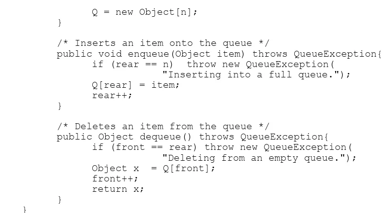
/* Inserts an item onto the queue */

public void enqueue(Object item) throws QueueException{ if (rear == n) throw new QueueException(

"Inserting into a full queue."); Q[rear] = item;

rear++; }

/* Deletes an item from the queue */

public Object dequeue() throws QueueException{ if (front == rear) throw new QueueException(

"Deleting from an empty queue."); Hence, there is a need to move the items to make room at the “rear-side” for future insertion. The method moveQueue implements this procedure. This could be invoked

There is a need to modify the implementation of enqueue to make use of moveQueue:

public void enqueue(Object item){

Linked allocation may also be used to represent a queue. It also makes use of nodes with fields INFO and LINK. The following figure shows a queue implemented as a linked list:

(43)

The node definition in chapter 1 will also be used here.

The queue is empty if front = null. In linked representation, since the queue grows dynamically, overflow will happen only when the program runs out of memory and dealing with that is beyond the scope of this topic.

The following Java code implements the linked representation of the ADT queue:

class LinkedQueue implements Queue{ queueNode front, rear;

/* Create an empty queue */ LinkedQueue(){

}

/* Create a queue with node n initially */ LinkedQueue(queueNode n){

front = n; rear = n; }

/* Inserts an item onto the queue */ public void enqueue(Object item){

queueNode n = new queueNode(item, null); if (front == null) {

/* Deletes an item from the queue */

public Object dequeue() throws QueueException{ Object x;

if (front == null) throw new QueueException

(44)

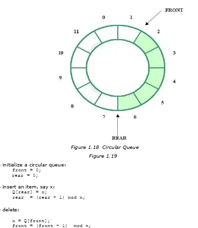
Figure 1.18 Circular Queue

Figure 1.19

To initialize a circular queue:

front = 0; rear = 0;

To insert an item, say x:

Q[rear] = x;

rear = (rear + 1) mod n;

To delete:

x = Q[front];

front = (front + 1) mod n;

We use the modulo function instead of performing an if test in incrementing rear and front. As insertions and deletions are done, the queue moves in a clockwise direction. If front catches up with rear, i.e., if front = rear, then we get an

empty queue. If rear catches up with front, a condition also indicated by front

= rear, then all cells are in use and we get a full queue. In order to avoid having the same relation signify two different conditions, we will not allow rear to catch up with front by considering the queue as full when exactly one free cell remains. Thus a full queue is indicated by:

front == (rear + 1) mod n

(45)

public void enqueue(Object item) throws QueueException{ if (front == (rear % n) + 1) throw new QueueException(

"Inserting into a full queue.");

if (front == rear) throw new QueueException(

"Deleting from an empty queue.");

Topological sorting is problem involving activity networks. It uses both sequential and link allocation techniques in which the linked queue is embedded in a sequential vector.

It is a process applied to partially ordered elements. The input is a set of pairs of partial ordering and the output is the list of elements, in which there is no element listed with its predecessor not yet in the output.

Partial ordering is defined as a relation between the elements of set S, denoted by ≼

which is read as 'precedes or equals'. The following are the properties of partial ordering

(46)

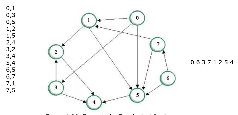
0,1

Figure 1.20 Example for Topological Sorting

0 6 3 7 1 2 5 4

3.5.1 The Algorithm

In coming up with the implementation of the algorithm, we must consider some components as discussed in chapter 1 – input, output and the algorithm proper.

• Input. A set of number pairs of the form (i, j) for each relation i ≼ j could represent the partial ordering of elements. The input pairs could be in any order.

• Output. The algorithm will come up with a linear sequence of items such that no item appears in the sequence before its direct predecessor.

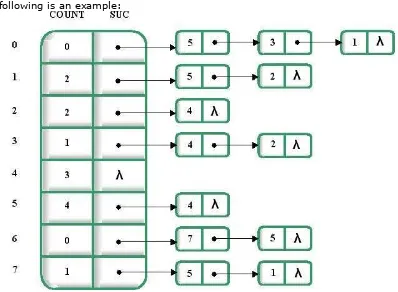
• Algorithm Proper. A requirement in topological sorting is not to output the items with which the predecessors are not yet in the output. To do this, there is a need to keep track of the number of predecessors for every item. A vector could be used for this purpose. Let's call this vector COUNT. When an item is placed in the output, the count of every successor of the item is decremented. If the count of an item is zero, or it becomes zero as a result of putting in the output all of its predecessors, that would be the time it is considered ready for output. To keep track of the successors, a linked list named SUC, with structure (INFO, LINK), will be used. INFO contains the label of the direct successor while LINK points to the next successor, if any.

The following shows the definition of the Node: class Node{

int info; Node link; }

The COUNT vector is initially set to 0 and the SUC vector to NULL. For every input pair (i, j),

(47)

and a new node is added to SUC(i):

Node newNode = new Node(); newNode.info = j;

newNode.link = SUC[i]; SUC[i] = newNode;

Figure 1.21 Adding a New Node

Figure 1.22

The following is an example:

(48)

Figure 1.24

Figure 1.25

To generate the output, which is a linear ordering of the objects such that no object appears in the sequence before its direct predecessors, we proceed as follows:

1. Look for an item, say k, with count of direct predecessors equal to zero, i.e., COUNT[k] == 0. Put k in the output.

2. Scan list of direct successors of k, and decrement the count of each such successor by 1.

3. Repeat steps 1 and 2 until all items are in the output.

To avoid having to go through the COUNT vector repeatedly as we look for objects with a count of zero, we will constitute all such objects into a linked queue. Initially, the queue will consist of items with no direct predecessors (there will always be at least one such item). Subsequently, each time that the count of direct predecessors of an item drops to zero, it is inserted into the queue, ready for output. Since for each item, say j, in the queue, the count is zero, we can now reuse COUNT[j] as a link field such that

COUNT[j] = k if k is the next item in the queue

= 0 if j is the rear element in the queue

Hence, we have an embedded linked queue in a sequential vector.

If the input to the algorithm is correct, i.e., if the input relations satisfy partial ordering, then the algorithm terminates when the queue is empty with all n objects placed in the output. If, on the other hand, partial ordering is violated such that there are objects which constitute one or more loops (for instance, 1≺2; 2≺3; 3≺4; 4≺1), then the algorithm still terminates, but objects comprising a loop will not be placed in the output.

This approach of topological sorting uses both sequential and linked allocation techniques, and the use of a linked queue that is embedded in a sequential vector.

3.6 Summary

• A queue is a linearly ordered set of elements obeying the first-in, first-out (FIFO) principle

• Two basic queue operations areinsertion at the rear and deletion at the front

• Queues have 2 implementations - sequential and linked

• In circular queues, there is no need to move the elements to make room for insertion

(49)

3.7 Lecture Exercise

1. Topological Sorting. Given the partial ordering of seven elements, how can they be arranged such that no element appears in the sequence before its direct predecessor?

a) (1,3), (2,4), (1,4), (3,5), (3,6), (3,7), (4,5), (4,7), (5,7), (6,7), (0,0) b) (1,2), (2,3), (3,6), (4,5), (4,7), ( 5,6), (5,7), (6,2), (0,0)

3.8 Programming Exercises

1. Create a multiple-queue implementation that co-exist in a single vector. Use Garwick's algorithm for the memory reallocation during overflow.

2. Write a Java program that implements the topological sorting algorithm.

3. Subject Scheduler using Topological Sorting.

Implement a subject scheduler using the topological sorting algorithm. The program shall prompt for an input file containing the subjects in the set and the partial ordering of subjects. A subject in the input file shall be of the form (number, subject) where

number is an integer assigned to the subject and subject is the course identifier [e.g. (1, CS 1)]. Every (number, subject) pair must be placed on a separate line in the input file. To terminate the input, use (0, 0). Prerequisites of subjects shall be retrieved also from the same file. A prerequisite definition must be of the form (i, j), one line per pair, where i is the number assigned to the prerequisite of subject numbered j. Also terminate the input using (0, 0).

The output is also a file where the name will be asked from the user. The output shall bear the semester number (just an auto-number from 1 to n) along with the subjects for the semester in table form.

For simplicity, we won’t consider here year level requisites and seasonal subjects.

Sample Input File Sample Output File

(50)

4 Binary Trees

4.1 Objectives

• Explain the basic concepts and definitions related to binary trees

• Identify the properties of a binary tree

• Enumerate the different typesof binary trees

• Discuss how binary trees are represented in computer memory

• Traverse binary trees using the three traversal algorithms: preorder, inorder, postorder

• Discuss binary tree traversal applications

• Use heaps and the heapsort algorithm to sort a set of elements

4.2 Introduction

Binary tree is an abstract data type that is hierarchical in structure. It is a collection of nodes which are either empty or consists of a root and two disjoint binary trees called the left and the right subtrees. It is similar to a tree in the sense that there is the concept of a root, leaves and branches. However, they differ in orientation since the root of a binary tree is the topmost element, in contrast to the bottommost element in a real tree.

Binary tree is most commonly used in searching, sorting, efficient encoding of strings, priority queues, decision tables and symbol tables.

4.3 Definitions and Related Concepts

A binary tree T has a special node, say r, which is called the root. Each node v of T that is different from r, has a parent node p. Node v is said to be a child (or son) of node p. A node can have at least zero (0) and at most two (2) children that can be classified as a

left child/son or right child/son. The subtree of T rooted at node v is the tree that has node v's children as its root. It is a left subtree if it is rooted at the left son of node

v or a right subtree if it is rooted at the right son of node v. The number of non-null subtrees of a node is called its degree. If a node has degree zero, it is classified as a

(51)

Figure 1.26 A Binary Tree

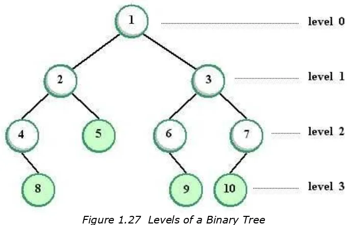
Level of a node refers to the distance of the node from the root. Hence, the root of the tree has level 0, its subtrees at level 1 and so on. The height or depth of a tree is the level of the bottommost nodes, which is also the length of the longest path from the root to any leaf. For example, the following binary tree has a height of 3:

Figure 1.27 Levels of a Binary Tree

Figure 1.28

(52)

A binary tree could be empty. If a binary tree has either zero or two children, it is classified as a proper binary tree. Thus, every proper binary tree has internal nodes with two children.

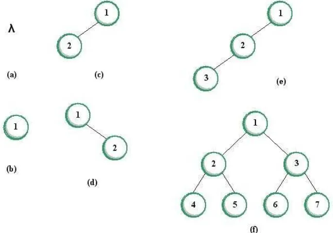
The following figure shows different they different types of binary tree: (a) shows an empty binary tree; (b) shows a binary tree with only one node, the root; (c) and (d) show trees with no right and left sons respectively; (e) shows a left-skewed binary tree while (f) shows a complete binary tree.

Figure 1.29 Different Types of Binary Tree

Figure 1.30

4.3.1 Properties of a Binary Tree

For a (proper) binary tree of depth k,

• The maximum number of nodes at level i is 2i_{, i} ≥ 0.

• The number of nodes is at least 2k + 1 and at most 2k+1

– 1.

• The number of external nodes is at least h+1 and at most 2k_. • The number of internal nodes is at least h and at most 2k_{– 1.}

• If no is the number of terminal nodes and n2 is the number of nodes of degree 2 in a

binary tree, then no = n2 + 1.

4.3.2 Types of Binary Tree

(53)

A right ( left ) skewed binary tree is a tree in which every node has no left (right)subtrees. For a given number of nodes, a left or right-skewed binary tree has the greatest depth.

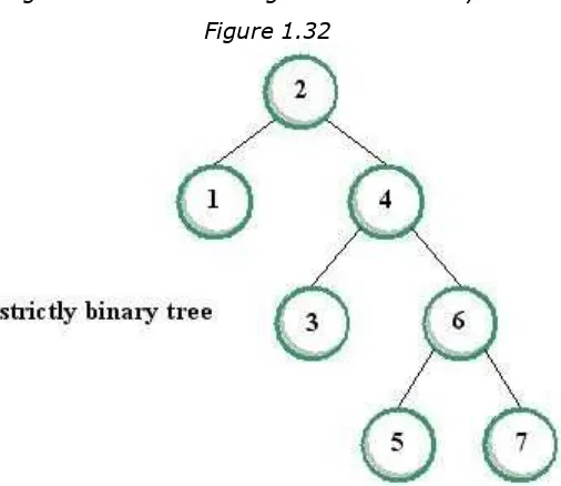
A strictly binary tree is a tree in which every node has either two subtrees or none at all.

Figure 1.31 Left and Right-Skewed Binary Trees

Figure 1.32

Figure 1.33 Strictly Binary Tree

(54)

Figure 1.34 Full Binary Tree

A complete binary tree is a tree which results when zero or more nodes are deleted from a full binary tree in reverse-level order, i.e. from right to left, bottom to top.

Figure 1.35 Complete Binary Tree

4.4 Representation of Binary Trees

The most 'natural' way to represent a binary tree in computer memory is to use link representation. The following figure shows the node structure of a binary tree using this representation:

(55)

Figure 1.37

The following Java class definition implements the above representation:

class BTNode { Object info;

BTNode left, right;

public BTNode(){ }

public BTNode(Object i) { info = i;

}

public BTNode(Object i, BTNode l, BTNode r) { info = i;

left = l; right = r; }

}

The following example shows the linked representation of a binary tree:

Figure 1.38 Linked Representation of a Binary Tree

Figure 1.39

Figure 1.40

In Java, the following class defines a binary tree:

class BinaryTree{

BTNode root;

BinaryTree(){ }

(56)

root = n; }

BinaryTree(BTNode n, BTNode left, BTNode right){ root = n;

root.left = left; root.right = right; }

}

4.5 Binary Tree Traversals

Computations in binary trees often involve traversals. Traversal is a procedure that visits the nodes of the binary tree in a linear fashion such that each node is visited exactly once, where visit is defined as performing computations local to the node.

There are three ways to traverse a tree: preorder, inorder, postorder. The prefix (pre, in and post) refers to the order in which the root of every subtree is visited.

4.5.1 Preorder Traversal

In preorder traversal of a binary tree, the root is visited first. Then the children are traversed recursively in the same manner. This traversal algorithm is useful for applications requiring listing of elements where the parents must always come before their children.

The Method:

If the binary tree is empty, do nothing (traversal done) Otherwise:

Visit the root.

Traverse the left subtree in preorder. Traverse the right subtree in preorder.

Figure 1.41 Preorder Traversal

(57)

In Java, add the following method to class BinaryTree:

/* Outputs the preorder listing of elements in this tree */ void preorder(){

if (root != null) {

System.out.println(root.info.toString()); new BinaryTree(root.left).preorder(); new BinaryTree(root.right).preorder(); }

}

4.5.2 Inorder Traversal

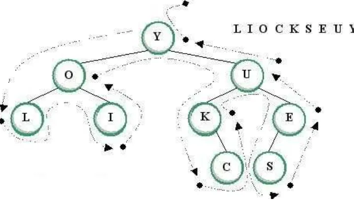
The inorder traversal of a binary tree can be informally defined as the “left-to-right” traversal of a binary tree. That is, the left subtree is recursively traversed in inorder, followed by a visit to its parent, then finished with recursive traversal of the right subtree also in inorder.

The Method:

Traverse the left subtree in inorder. Visit the root.

Traverse the right subtree in inorder.

Figure 1.43 Inorder Traversal

Figure 1.44

/* Outputs the inorder listing of elements in this tree */ void inorder(){

if (root != null) {

(58)

} }

4.5.3 Postorder Traversal

Postorder traversal is the opposite of preorder, that is, it recursively traverses the children first before their parents.

The Method:

Traverse the left subtree in postorder. Traverse the right subtree in postorder. Visit the root.

Figure 1.45 Postorder Traversal

Figure 1.46

/* Outputs the postorder listing of elements in this tree */ void postorder(){

if (root != null) {

new BinaryTree(root.left).postorder(); new BinaryTree(root.right).postorder(); System.out.println(root.info.toString()); }

}

(59)

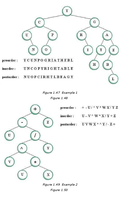
Figure 1.47 Example 1

Figure 1.48

Figure 1.49 Example 2

(60)

4.6 Applications of Binary Tree Traversals

Binary tree traversals have several applications. In this section, two applications will be covered: duplication of a binary tree and checking equivalence of two binary trees.

4.6.1 Duplicating a Binary Tree

There are instances that a duplicate of an existing binary tree would be needed for computation. To do this, the following algorithm to copy an existing binary tree can be used:

1. Traverse the left subtree of node α in postorder and make a copy of it 2. Traverse the right subtree of node α in postorder and make a copy of it 3. Make a copy of node α and attach copies of its left and right subtrees

The following Java method of the BinaryTree class implements copy:

/* Copies this tree and returns the root of the duplicate */ BTNode copy(){

newRoot = new BTNode(root.info, newLeft, newRight);

return newRoot;

}

return null; }

4.6.2 Equivalence of Two Binary Trees

Two binary trees are equivalent if one is an exact duplicate of the other. The following is the algorithm to check equivalence of two binary trees:

1. Check whether node α and node α contain the same data

2. Traverse the left subtrees of node α and node α in preorder and check whether they are equivalent

3. Traverse the right subtrees of node α and node α in preorder and check whether they are equivalent

The following code snippet, which is a method of BinaryTree, implements this algorithm:

/* Compare another tree t2 if it's equivalent to this tree */ boolean equivalent(BinaryTree t2){

boolean answer = false;

| Komputasi | Suatu Permulaan

Data

Structures

Table of Contents

1 Basic Concepts and Notations

1.1 Objectives

1.2 Introduction

1.3 Problem Solving Process

1.4 Data Type, Abstract Data Type and Data

Structure

1.5 Algorithm

1.6 Addressing Methods

1.6.1 Computed Addressing Method

1.6.2 Link Addressing Method

1.7 Mathematical Functions

1.8.1 Algorithm Efficiency

The Big-Oh Notation

1.8.3 Analysis of Algorithms

1.9 Summary

1.10 Lecture Exercises

2 Stacks

2.1 Objectives

2.2 Introduction

2.3 Operations

2.4 Sequential Representation

2.6 Sample Application: Pattern Recognition

Problem

-2.7 Advanced Topics on Stacks

2.7.1 Multiple Stacks using One-Dimensional Array

2.7.2 Reallocating Memory at Stack Overflow

2.8 Summary

2.9 Lecture Exercises

3 Queues

3.1 Objectives

3.2 Introduction

3.3 Representation of Queues

3.3.1 Sequential Representation

3.5.1 The Algorithm

3.6 Summary

3.7 Lecture Exercise

3.8 Programming Exercises

4 Binary Trees

4.1 Objectives

4.2 Introduction

4.3 Definitions and Related Concepts

4.3.1 Properties of a Binary Tree

4.3.2 Types of Binary Tree

4.4 Representation of Binary Trees

4.5 Binary Tree Traversals

4.5.1 Preorder Traversal

4.5.2 Inorder Traversal

4.5.3 Postorder Traversal

4.6 Applications of Binary Tree Traversals

4.6.1 Duplicating a Binary Tree

4.6.2 Equivalence of Two Binary Trees