Full Terms & Conditions of access and use can be found at
http://www.tandfonline.com/action/journalInformation?journalCode=cbie20
Bulletin of Indonesian Economic Studies
ISSN: 0007-4918 (Print) 1472-7234 (Online) Journal homepage: http://www.tandfonline.com/loi/cbie20
Block Rate Pricing of Water in Indonesia: An
Analysis of Welfare Effects
Piet Rietveld , Jan Rouwendal & Bert Zwart
To cite this article:
Piet Rietveld , Jan Rouwendal & Bert Zwart (2000) Block Rate Pricing of
Water in Indonesia: An Analysis of Welfare Effects, Bulletin of Indonesian Economic Studies,
36:3, 73-92
To link to this article:
http://dx.doi.org/10.1080/00074910012331338983
Published online: 18 Aug 2006.
Submit your article to this journal
Article views: 119
View related articles
BLOCK RATE PRICING OF
WATER IN INDONESIA:
AN ANALYSIS OF WELFARE EFFECTS
Piet Rietveld
Vrije Universiteit Amsterdam
Jan Rouwendal
Landbouwuniversiteit Wageningen
Bert Zwart*
Vrije Universiteit Amsterdam
INTRODUCTION
In 1994, about 40% of the Indonesian urban population (27 million people) had access to piped drinking water, while in rural areas, where alternative water sources such as wells and rivers are more abundant, it was available to about 10% of the population (10 million people). The quality of the piped water system is rather low: water must be boiled because it is not safe to drink; about 40% of it disappears because of leakages; and supply is frequently interrupted in many places.
Piped water in Indonesia is supplied by regional water companies (PDAM: Perusahaan Daerah Air Minum), a decentralised government monopoly. There are about 300 PDAMs in the country. Their profits usually form a small part of the revenue of regional governments (kabupaten and kotamadya), but in some cases a PDAM provides an important source of income for the local administration (IRC 1997). Data from PDAM reports indicate that 70% of all PDAMs have negative net revenues when depreciation is taken into account. Thus in the majority of cases it is only when depreciation costs are not accounted for in a proper way that a money flow can occur between the PDAM and the regional government.
In terms of privatisation, clean water has lagged behind other services such as transport (toll roads), electricity and telecommunications, where private investors have played an important role. Large investments would be needed to bring about a substantial increase in the penetration of piped drinking water. The public sector seems unable to realise such an intensive investment program, and private sector involvement will be necessary to speed up investments in water supply. One of the bottlenecks appears to be the pricing of water. Governments are reported to keep prices low enough to be affordable to as many households as possible (IRC 1997), which reduces the attractiveness of water supply as an investment opportunity for the private sector.
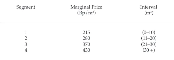
Each PDAM has its own system of prices, with various schemes for households, commercial activities and the public sector. A special feature of the pricing system for households that is shared by the various PDAMs is that it is progressive: the larger the volumes consumed, the higher the marginal price paid. Table 1 gives an example of the pricing structure of the PDAM of the city of Salatiga in Central Java. The table shows that the price paid for the first cubic metre (m3) of water (Rp 215/m3) is only half
that paid for each additional m3 when large quantities of water are
The progressive price structure used by Indonesian PDAMs is a special example of multi-part pricing, a practice whose origins are traced in Pigou (1920), in which the marginal price of a good is different for various levels of demand. This system is only practicable when the consumer can be identified and resale is difficult. Both conditions are met in the case of water demand. In the well known textbook example, a profit maximising monopolist would introduce a price structure with a variable part to cover the marginal cost and a fixed part to absorb the consumer surplus (Coase 1946; Varian 1989; Brauetigam 1989; Gravelle and Rees 1992). This form of pricing is often used in sectors with large economies of scale leading to high overhead costs, but its use is not restricted to such cases: it could arise with any cost structure. This pricing strategy is consistent with maximising both profits and efficiency. Efficiency is guaranteed, since the price is equal to the marginal cost, so that the well known problem of underconsumption due to a high monopolistic price is avoided. Profits are maximised via introduction of the fixed charge.1 Thus any problems
one might have with this form of monopolistic price setting would have to be with the equity aspect (fairness of income distribution) rather than with efficiency. This standard form of multi-part pricing leads to a
decreasing average price being paid by consumers: the more they consume, the lower the average price. In the Indonesian case the opposite occurs: the price structure used here implies an increasing average price.
We conclude from the above that profit maximisation is apparently not the objective of Indonesian public water companies. Why then do these public monopolists apply a progressive price structure? A basic reason is that PDAMs wish to promote equity: high-income households
TABLE 1 Price Structure with Increasing Marginal Prices, Salatiga, 1994
Segment Marginal Price Interval
(Rp/m3) (m3)
1 215 (0–10)
2 280 (11–20)
3 370 (21–30)
consuming large volumes of water pay higher prices than households consuming small quantities. PDAMs are conceived of as firms with a social mission, which apply cross-subsidies from rich to poor households (IRC 1997).
There is a further possible reason for the choice of pricing structure. Water companies may wish to avoid the situation where households share a connection to the piped water system; as we will see below a certain proportion of households have adopted the practice of using a connection jointly with their neighbours. By taking individual connections, households face lower marginal prices, but this has, of course, to be traded off against the fact that the installation fee must be paid twice.2
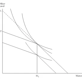
The application of a progressive system of block rate pricing has special consequences in terms of economic theory and econometric estimation. Figure 1 illustrates the kinked budget constraint of consumers facing block rate pricing, in which water purchases in excess of the kink at Wk are at a higher price than purchases up to that level. Given strictly convex budget constraints like those shown here, a substantial number of consumers may be expected to find their optimal consumption bundle at the kink—i.e. consuming Wk of water—even though they have different
utility functions or different income levels. (Figure 1 is explained in detail below.)
From an econometric viewpoint the problem with kinked or non-linear budget constraints is that the marginal price paid becomes a function of the quantity consumed. Thus when one estimates a demand function one cannot apply the standard approach in which quantity consumed is the dependent variable and marginal price is an independent variable. A treatment of these estimation problems can be found in a study by Burtless and Hausman (1978), who have developed econometric methods for analysing piece-wise linear constraints. The literature is reviewed in Moffitt (1986, 1990), and an econometric application is provided by Hewitt and Hanemann (1995).
to be efficient (i.e. when the price equals the marginal cost), whereas the progressive price structure used by the water companies does not have this potential.
The reason we address the equity issue is that the progressive price structure may be expected to perform better in equity terms than the two-part price system with a uniform marginal price, because it would allow poor households that consume little water to pay lower prices. The question is whether the progressive price system has sufficient positive equity effects to make it an attractive alternative to a potentially more efficient uniform pricing strategy (assuming that price equals marginal cost).
FIGURE 1 Consumption Optima for Individuals with Different Preferences and Incomes under Block Rate Pricing of Watera
yv
y
Wk Water
Other good
In the present paper we estimate the demand function for piped water consumed by urban households, using the econometric techniques mentioned above. We report on some data issues before discussing the estimation results. On the basis of the demand function, a welfare economic analysis is then carried out in order to determine whether a progressive price system is advisable from an equity perspective. The analysis is based on a household survey conducted in Salatiga.
DATA
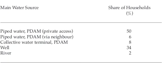
The study carried out in Salatiga, a medium-sized city in Central Java with about 100,000 inhabitants, suggests that about 50% of the households have direct access to piped water (table 2).
A private connection to the piped water system is not the only way PDAM services are consumed: 6% of households get their water from a neighbour who has a private connection, and 8% obtain PDAM water via a community water terminal.3 The rest of the population gets its water
from wells and rivers. Water vendors play a negligible role in Salatiga, although they are significant in large cities like Jakarta, where the supply of water of sufficient quality from wells and rivers is small (Crane and Daniere 1996). The figures shown in table 2 relate to the main water source; some households use more than one source. The data presented in the table are based on a sample of 951 households. In our analysis of demand for piped water we focus on the group of 50% having a private connection, because it is only for this group that we know the quantities of water consumed.
TABLE 2 Distribution of Households According to Main Water Source, Salatiga, 1994
Main Water Source Share of Households
(%)
Piped water, PDAM (private access) 50
Piped water, PDAM (via neighbour) 6
Collective water terminal, PDAM 8
Well 34
River 2
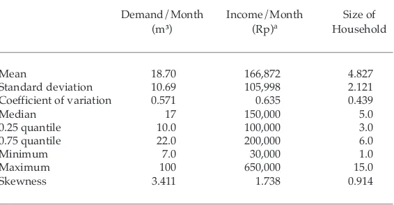
Table 3 presents some descriptive statistics of relevant variables, and table 4 examines some relationships among these variables. It can be seen that the distributions of water demand and income are highly skewed to the right. The correlation between demand and income is low, as is that between household size and income.
Some results on water demand not found in the table are of interest. About 37% of the data are equal to 10, 20 or 30 m3/month, and thus lie on
one of the kinks. This fact may be due to rounding errors, but gives some extra support to the use of the Burtless and Hausman model.
TABLE 3 Descriptive Statistics of Demand Related Variables, Salatiga Water Study, 1994
Demand/Month Income/Month Size of
(m3) (Rp)a Household
Mean 18.70 166,872 4.827
Standard deviation 10.69 105,998 2.121
Coefficient of variation 0.571 0.635 0.439
Median 17 150,000 5.0
0.25 quantile 10.0 100,000 3.0
0.75 quantile 22.0 200,000 6.0
Minimum 7.0 30,000 1.0
Maximum 100 650,000 15.0
Skewness 3.411 1.738 0.914
aIn March 1994, the exchange rate was approximately Rp 2,000/$.
TABLE 4 Correlations between Demand Related Variables, Salatiga Water Study, 1994
Income Size of Household
Demand 0.060 0.438
ESTIMATION RESULTS
To estimate water demand, we use the Burtless and Hausman method (1978) for analysing choice behaviour under piece-wise linear constraints.4
The price structure shown in table 1 would lead to a specification with three kinks, at 10, 20 and 30 m3. However, we make the following
extension. Since demand is bounded from below (by zero) and above (by budget restriction), we add two kinks to the boundaries of the interval of feasible demand. Table 1 contains the values of the kinks, segments, and corresponding marginal prices pm,1, …, pm,4.
The following specification for the logarithm of water demand is used in the estimation procedure:
Virtual income is defined as the income of a household conditioned on the marginal price it pays for water. In figure 1, virtual income is measured along the vertical axis: for households consuming less than Wk units of
water, virtual income is equal to actual income. However, for those consuming more than Wk units virtual income is higher, as indicated by the intersection of the extended steeper segment of the budget constraint and the vertical axis. Virtual income is higher than actual income for such households (measured in terms of the other good) because the lower infra-marginal price paid for the first Wk units of water permits greater expenditure on the other good than would be possible at the higher (uniform) water price. For further details on the use of virtual incomes in this context we refer to Moffitt (1986). The parameters β, γ and δ are parameters to be estimated. The parameter α is a random coefficient that is introduced to take care of heterogeneity among households. It reflects taste differences: some households are more inclined to consume water than others. The parameter ε represents a common measurement error. In standard econometric estimations of demand functions, α and ε cannot be distinguished. However, in the present context of kinked budget constraints, the two stochastic components are distinguishable (Moffitt 1990).
Water consumption depends strongly on household size: the coefficient of 0.526 means, for example, that in a household with three persons, consumption is 24% higher than in one with two persons [(3/2).526 = 1.24]. This result is no surprise, given the rather high correlation
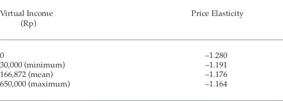
between water consumption and household size shown in table 2. The value of the coefficient of D differs significantly from zero when a likelihood ratio test is performed. Water demand is 22% lower when an extra water source is available. The only coefficient that does not differ significantly from zero is that for virtual income yv. This is also the conclusion when the product ln(pm)ln(yv) is left out of the specification. This product term is significant and adds extra richness to the model, in the sense that the price elasticity is no longer constant. Table 6 shows various values of the price elasticity for a given value of (virtual) income. The mean price elasticity is –1.176. Very low-income households appear to be slightly more sensitive to price increases than higher-income households. Thus we arrive at the conclusion that water demand in Salatiga has a strong dependence on the price of water. The values of the
TABLE 5 Household Water Demand: Estimation Results, Salatiga, 1994
ln(q) = 8.764 + 0.526 ln(H) – 0.220 D – 1.280 ln (pm) + 0.501 10–6 ln(y
v) + 8.604 10 –3 ln(p
m)ln(yv) (1.22) (0.099) (0.142) (0.235) (0.348)10–6 (1.164)10–3
α ~ N( 0, 0.5582 ) ε ~ N( 0, 0.0202 )
(0.036) (0.0052)
Log-likelihood = –681.06
TABLE 6 Price Elasticity as a Function of Income
Virtual Income Price Elasticity
(Rp)
0 –1.280
30,000 (minimum) –1.191
166,872 (mean) –1.176
price elasticities obtained here are higher (in an absolute sense) than the range of about –0.3 to –0.9 mentioned by Nieswiadomy and Molina (1989) for the US. On the other hand Hewitt and Hanemann (1995) arrive at an elasticity of about –1.6 for households in Texas, and mention some other studies yielding elasticities of water demand clearly higher than one (in an absolute sense). Most of the studies in this field relate to the US, where indoor water consumption is thought to be rather price independent, whereas outdoor consumption (for watering lawns) is much more price dependent (other studies pertain to Europe and Australia). This context cannot be easily transferred to a developing country such as Indonesia, where lawn watering is not usual. Espey et al. (1997) report in a recent survey of the literature that they found elasticities between –0.02 and –3.33, averaging –0.51. We conclude therefore that our estimate is rather high compared with what most of the studies find, but is not exceptionally high.
Another advantage that emerges when the product term is added is that income effects are clearly positive. The income elasticity has a mean of 0.049 and ranges between 0.046 and 0.052.5
The rather limited role of income in our estimation result may arise from our considering only households that already have a PDAM connection. The decision to have such a connection probably depends strongly on income: to obtain a connection, an installation fee of about Rp 200,000 must be paid. In reality, the figure may be considerably higher: waiting lists are long, and in order to expedite a connection it is often necessary to bribe PDAM employees.
The installation fee is rather high in relation to monthly expenses. It would amount to at least the equivalent of Rp 2,500 per month (assuming a 15% interest rate), and this would more than double the cost of water to a household consuming at a low level of 10 m3/month. For the median
household (in terms of water consumption), the installation fee would still be some 40% of total water-related expenditures. This high fee is one reason households may decide to cooperate with their neighbours by having only one connection for two or more households.
One would expect a positive correlation between the income level of households and whether they have a PDAM connection, because many low-income households will not be able to afford the fixed costs involved. In addition, one would expect supply from the water network to be limited in areas with many low-income households.
In the present paper we did not analyse the impact of the installation fee on the decision about whether to be connected to the water network. This decision depends on two factors: supply and demand. A household can only be connected when two conditions are fulfilled: a pipeline is present, and the household is interested in being connected. If a household is not connected this may be a matter not of choice, but of the lack of a pipeline. Unfortunately, data on ownership of a PDAM connection could not be linked to data on the presence of a pipeline in the local area, so a meaningful analysis of the decision to be connected was not feasible.
WELFARE EFFECTS OF UNIFYING THE RATE STRUCTURE
One justification that PDAMs give for the block rate pricing structure relates to equity. The system favours households with small budgets and—presumably—low water consumption, because the marginal price is relatively low for small consumption levels. It appears from our estimation results that income has a significant though small effect on water consumption, whereas household size has a more substantial influence. This implies that the main consequence of the current rate structure may well be that larger households pay a higher marginal price than small households do, but that income is an unimportant determinant of the marginal price. Such an effect is almost surely unintended, and probably not desired, by the authorities that determine the price schedule. It is therefore of some interest to investigate the welfare consequences of unifying the rate structure.
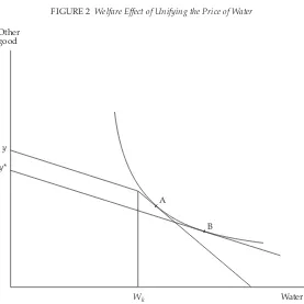
The appropriate tool for doing so is the expenditure function, or the closely related indirect utility function. Either of these allows us to determine the compensating variation, which is the change in income that is required to keep a household at the same indifference curve after a change in the price schedule for water has occurred. However, the expenditure function and the indirect utility function that are associated with the demand function estimated here are unknown, and the method proposed by Hausman (1981) does not lead to an (easily) solvable differential equation. We therefore make use of the procedure developed by Vartia (1983), which requires only knowledge of the ordinary (Marshallian) demand functions (see also Johansson 1991).6
(relative) uniform price for water. The straight line that touches the indifference curve at this point is the budget constraint that would lead the utility maximising individual to choose B as the optimum consumption bundle. The income implied by this budget line, y*
(measured in terms of the other good), is the income that would be needed to make the consumer indifferent between the current rate structure and the uniform price. The difference between actual income, y, and y* is the compensating variation. If the compensating variation is negative—which will be the case if the new uniform price is above a certain level—a higher income will be needed to keep the consumer on the same indifference curve after the rate structure is unified. If it is positive, as in the case shown in figure 2, a lower income would suffice. Clearly, in the former case the change is to the disadvantage of the household, in the latter to its benefit.
FIGURE 2 Welfare Effect of Unifying the Price of Water
y
y*
Wk Water
Other good
A
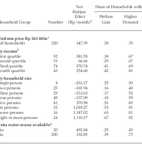
The uniform price can be set at various levels. As a first example we consider the case that the uniform price is set equal to the current average price paid by households (total revenue divided by total quantity currently sold). This price equals Rp 263.40 per m3. The welfare effect on
households, measured in terms of the compensating variation, is given in table 7. The aggregate effect of the uniform price is that total water consumption increases: the fall in the number of households with low consumption levels is more than offset by the increase in the number of households with high consumption levels. The share of households that consume more under the uniform price is 70%. Not all of these households experience a welfare gain. As can be inferred easily from figure 2, depending on the utility function of the household, an increase in water consumption resulting from the change in price system can lead to both a positive and a negative compensating variation). The share of households with a positive compensating variation equals 38%, so the majority of the households have a negative compensating variation. The average welfare gain is positive, however. Thus, there is a rather large group of households that experience a small welfare loss and a smaller group of households that experience a relatively large welfare gain.
A comparison of the welfare effects for various household classes yields interesting insights. The differences between the various income groups are quite small. For example, when one compares the highest and the lowest quartile, the shares of households that benefit from the uniform price are quite similar (42% versus 38%), and the net benefit of the low-income group is even higher than that of the high-low-income group. Our analysis reveals that there is no systematic pattern according to which high-income households benefit from the introduction of uniform prices. This is an important conclusion, because it destroys the main argument in favour of the prevailing price structure—the equity argument that high-income households with high consumption levels should pay part of the bill for low-income households. The main reason why the equity mechanism does not work is that income is only weakly related to water consumption, as has been demonstrated in tables 4 and 5.
A much more systematic pattern of effects is found when we consider
variable of water demand. Large households tend to consume more water and will therefore gain from the introduction of a uniform price that is lower than the current marginal price they pay. We conclude that the progressive block rate system is beneficial for small households, but these are not necessarily low-income households. As indicated in table 4, the correlation between household size and household income is rather low.
TABLE 7 Welfare Effects of Unifying the Rate Structure: Average Price Remains Unchanged
Net Share of Households with Welfare
Effect Welfare Higher Household Group Number (Rp/month)a Gain Demand
Uniform price Rp 263.40/m3
All households 220 347.39 .38 .70
By incomeb
First quartile 52 381.55 .38 .67
Second quartile 51 66.66 .29 .67
Third quartile 74 570.74 .41 .69
Fourth quartile 43 254.68 .42 .81
By household size
Single person 4 –233.17 .25 .50
Two persons 25 –101.94 .16 .40
Three persons 29 –212.63 .17 .52
Four persons 49 –137.09 .18 .59
Five persons 41 370.98 .51 .85
Six persons 32 1,018.27 .53 .91
Seven persons 16 1,147.02 .63 .81
Eight or more persons 24 1,110.17 .67 .92
Extra water source available?
Yes 20 492.84 .25 .45
No 200 332.85 .39 .73
aAverage compensating variation for the relevant group.
bDifferences in the number of households per quartile are due to a large number
If the welfare analysis were carried out on the basis of individuals instead of households, some results would change markedly. The overrepresentation of large households in the group of households with a positive net benefit implies, for example, that if the individual were the unit a much higher number of units would have net benefits: whereas 38% of households have a welfare gain, more than 50% of individuals would have a welfare gain.
The effect of the availability of an extra water source is somewhat unexpected: households with an extra water source have a higher net welfare gain than other households. The probable explanation is that the households with an extra source are often large households.
The results in table 7 are confined to direct welfare effects related to the consumption of water. Another effect to be considered concerns the profit of the water company. Given the economies of scale, increased water consumption can probably be realised against rather low marginal costs. Although we do not know the level of the marginal costs, it is quite possible that they are lower than the uniform price posited here. The consequence would be an increase in the profits of the water company, which would be used for public expenditures from which the households would benefit. Thus the figures in table 7 probably contain underestimates of the net welfare changes.
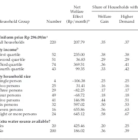
Since we do not know the marginal cost of water production, it is not possible to use this as a benchmark in our welfare analysis. Another level of the uniform price that is of some interest in this study is the level where aggregate demand would remain unchanged. This level is estimated to be Rp 296.1 per m3. The advantage of using this price level
Table 8 shows that with a price level where total demand remains unchanged, 37% of all households will consume more water, and the rest will consume the same amount or less. There is a net welfare gain to 35% of households. The average net welfare effect is positive: compared with table 7, the compensating variation decreases because of the higher price,
TABLE 8 Welfare Effects of Unifying the Rate Structure: Total Demand Remains Unchanged
Net Share of Households with Welfare
Effect Welfare Higher Household Group Number (Rp/month)a Gain Demand
Uniform price Rp 296.09/m3
All households 220 207.79 .35 .37
By incomeb
First quartile 52 235.00 .38 .38
Second quartile 51 36.83 .29 .29
Third quartile 74 369.51 .36 .41
Fourth quartile 43 99.35 .33 .42
By household size
Single person 4 –106.38 .25 .25
Two persons 25 31.41 .16 .16
Three persons 29 –82.25 .17 .17
Four persons 49 –68.72 .18 .18
Five persons 41 146.98 .44 .51
Six persons 32 597.02 .50 .53
Seven persons 16 655.86 .56 .63
Eight or more persons 24 645.12 .58 .67
Extra water source available?
Yes 20 425.46 .20 .25
No 200 186.02 .36 .39
aSee table 7, note a.
but households benefit from higher public expenditures made possible by the increased profits of the water company. Since we assume that these public expenditures are distributed equally among households, it is no surprise that the change in welfare position of the large households is smaller with the higher than with the lower price (compare tables 8 and 7). For the rest, the distributional patterns related to the two uniform prices are rather similar.
Tables 7 and 8 show two examples in which the transition from the progressive price structure to the uniform price is welfare improving for the average consumer. This is consistent with the suggestion above that a progressive price system performs badly in terms of efficiency, because it leads to a loss of consumer surplus among households with high water demand. The tables also show that the social equity effects of the change in price structure are limited. The shifts in the welfare positions of income groups are relatively small. For household size groups the shifts are much larger, but this is not a sensitive issue from an equity viewpoint, since size is not closely correlated with income.
One might of course consider other uniform prices, possibly in combination with a fixed access charge per month, not dependent on consumption. For an assessment of the equity aspects of pricing, this will not add much to the insights already obtained in tables 7 and 8. And for an analysis of the efficiency of other uniform prices we would need data on the marginal costs of water supply. Note also that, since the present price system already contains a fixed installation fee, it does not make much sense to add a fixed monthly access charge, because the two are entirely interchangeable.
CONCLUSIONS
The majority of Indonesian households do not have an own connection to piped water. Substantial resources would be needed for large-scale investments in this sector. Private sector involvement has been insignificant in Indonesia’s water supply thus far. A bottleneck for private sector involvement appears to be the structure and level of water prices. The progressive price structure being used leads to cross-subsidies between households with large and small consumption levels.
A two-part pricing structure with a uniform price equal to the marginal cost of production, combined with a fixed access charge, would lead to an efficient allocation. A progressive price structure cannot be made compatible with the efficiency criterion, but it might outperform the two-part price structure from an equity viewpoint. We therefore focus in this paper on equity considerations. We note that installation costs present a barrier to poor households. Thus the price structure of the PDAMs becomes a strange mixture of progressive and regressive elements: it is difficult to understand why equity considerations suddenly matter in pricing policy after households have been charged a high installation fee which discourages poor households from obtaining a PDAM connection.
In order to address the equity issue, we first estimate the demand functions for water. The estimation results indicate a large price elasticity (in absolute value) and a small income elasticity. The price elasticity is decreasing in income (in absolute value). The average price elasticity is about –1.17. Our analysis shows that replacing the block rate structure with a uniform marginal price leads on average to an increase in household welfare. The principal beneficiaries of a uniform price are large
NOTES
* The authors are grateful to Prapto Yuwono and Supramono for useful advice and for making the data available. They also thank two anonymous referees for constructive comments. André Oosterman provided background information on PDAMs.
1 This result holds true with first degree price discrimination, where the supplier has perfect knowledge of each consumer’s willingness to pay. When there is no such perfect information, efficiency and profit maximisation usually do not go together (Varian 1989).
2 A possible additional reason for the choice of price structure relates to the objective of promoting economical water use by households: the high price for large volumes stimulates them to reduce consumption. Such a consideration arises in the pricing policies of public utilities in some countries, but in Indonesia, where environmental issues generally receive low policy priority, it probably does not play a role.
3 Consumers pay through the leader of their community, and the price is lower than would be paid for an ordinary connection.
4 Details of the econometric analysis are available from the authors on request; contact <[email protected]>.
5 The mean income elasticity is defined as the income elasticity for the mean marginal price observed in the sample.
6 In our case, the system of demand functions consists of two equations: one for water, the other for a (Hicksian) composite consumption good. All conditions required by Vartia’s method are met if the demand equation for water meets the Slutsky condition. A proof is available upon request from the authors. The method we use yields a slightly more accurate estimation of the compensating variation than the alternative method of Willig (1976).
REFERENCES
Brauetigam, R.R. (1989), ‘Optimal Policies for Natural Monopolies’, in R. Schmalensee and R.D. Willig (eds), Handbook of Industrial Organization, North Holland, Amsterdam: 1,289–346.
Burtless, G., and J. Hausman (1978), ‘The Effect of Taxation on Labour Supply: Evaluating the Gary Income Maintenance Experiment’, Journal of Political Economy 86: 1,103–30.
Coase, R. (1946), ‘The Marginal Cost Controversy’, Economica 13: 169–89. Crane, R., and A. Daniere (1996), ‘Measuring Access to Basic Services in Global
Cities: Descriptive and Behavioral Approaches, Journal of the American Planning Association 62 (2): 203–21.
Gravelle, H., and R. Rees (1992), Micro-economics, Longman, London.
Hausman, J.A. (1981), ‘Exact Consumer’s Surplus and Deadweight Loss’, American Economic Review 71: 662–76.
Hewitt, J.A., and W.M. Hanemann (1995), ‘A Discrete/Continuous Approach to Residential Water Demand under Block Rate Pricing’, Land Economics 71: 173–92.
IRC (Indonesia Research Consult) (1997), The Water Industry in Indonesia: Opportunities for the Private Sector, Jakarta.
Johansson, P-O. (1991), The Economic Theory and Measurement of Environmental Benefits, Cambridge University Press, Cambridge.
Moffitt, R. (1986), ‘The Econometrics of Piecewise-Linear Budget Constraints’, Journal of Business and Economic Statistics 4 (3): 317–28.
—— (1990), ‘The Econometrics of Kinked Budget Constraints’, Journal of Economic Perspectives 4 (2): 119–39.
Nieswiadomy, M.L., and D.J. Molina (1989), ‘Comparing Residential Water Demand Estimates under Decreasing and Increasing Block Rates Using Household Data’, Land Economics 65: 280–9.
PDAM (Perusahaan Daerah Air Minum) (1997), Financial Report 1996, Jakarta. Pigou, A.C. (1920), The Economics of Welfare, MacMillan, London.
Supramono and B. Wijayanto (1995), Permintaan Riil Prasarana Kota [Demand for Urban Infrastructure], Universitas Kristen Satya Wacana, Salatiga. Varian, H.R. (1989), ‘Price Discrimination’, in R. Schmalensee and R.D. Willig (eds),
Handbook of Industrial Organization, North Holland, Amsterdam: 597–654. Vartia, Y.O. (1983), ‘Efficient Methods of Measuring Welfare Change and
Compensated Income in Terms of Ordinary Demand Functions’, Econometrica 51: 79–98.