Full Terms & Conditions of access and use can be found at
http://www.tandfonline.com/action/journalInformation?journalCode=ubes20
Download by: [Universitas Maritim Raja Ali Haji] Date: 13 January 2016, At: 01:07
Journal of Business & Economic Statistics
ISSN: 0735-0015 (Print) 1537-2707 (Online) Journal homepage: http://www.tandfonline.com/loi/ubes20
The Estimation of Dynamic Bivariate Mixture
Models
Toshiaki Watanabe
To cite this article: Toshiaki Watanabe (2003) The Estimation of Dynamic Bivariate
Mixture Models, Journal of Business & Economic Statistics, 21:4, 577-580, DOI: 10.1198/073500103288619304
To link to this article: http://dx.doi.org/10.1198/073500103288619304
Published online: 01 Jan 2012.
Submit your article to this journal
Article views: 40
The Estimation of Dynamic Bivariate Mixture
Models: Reply to Liesenfeld
and Richard Comments
Toshiaki WATANABE
Faculty of Economics, Tokyo Metropolitan University, 1-1 Minami Ohsawa, Hachioji-shi, Tokyo 192-0397, Japan (twatanab@bcomp.metro-u.ac.jp)
Watanabe estimated the dynamic bivariate mixture models introduced by Tauchen and Pitts and modied by Andersen using a Bayesian method via Markov chain Monte Carlo techniques. Based on a maximum likelihood method via efcient importance sampling, Liesenfeld and Richard obtained estimates that are signicantly different from those of Watanabe. This note corrects the error in the multimove sampler used by Watanabe and reproduces all analyses in the work of Watanabe using a corrected multimove sampler. The estimates using the correct multimove sampler are found to be close to those obtained by Liesenfeld and Richard.
KEY WORDS: Efcient importance sampling; Latent variable; Markov chain Monte Carlo; Multimove sampler.
1. INTRODUCTION
Liesenfeld and Richard (2002) have found that the results of Watanabe (2000) are inconsistent with those in the previ-ous literature. Specically, Watanabe’s estimates of the persis-tence in the latent variable in the the dynamic bivariate mix-ture models are very close to that in the stochastic volatility model, whereas Andersen (1996) and Liesenfeld (1998) found that the persistence in the latent variable drops signicantly in the the dynamic bivariate mixture models. Using the data set of Watanabe (2000), Liesenfeld and Richard estimated the sto-chastic volatility model and the Tauchen and Pitts (1983) model based on the maximum likelihood method via an efcient im-portance sampling procedure. Their estimate of the persistence in the latent variable in the Tauchen and Pitts model is much smaller than that in the stochastic volatility model and signi-cantly different from that of Watanabe. Their result has identi-ed an error in the work of Watanabe (2000). This note corrects the error in the multimove sampler used by Watanabe and re-produces all analyses in his article (Watanabe 2000) using a corrected multimove sampler. The obtained estimate of the per-sistence in the latent variables in the Tauchen and Pitts (1983) model is much smaller than that in the stochastic volatility model and is close to that obtained by Liesenfeld and Richard (2002).
2. A CORRECT MULTIMOVE SAMPLER
This section explains the error in the multimove sampler used by Watanabe (2000) and corrects it. For this purpose, it sufces to consider the Tauchen and Pitts (1983) model, al-though Watanabe also estimated the stochastic volatility model, the Andersen (1996) model, and the extended Tauchen and Pitts (1983) model. The Tauchen and Pitts model used by Watanabe is given by
RtjIt»N.0; ¾r2It/; (1) VtjIt»N.¹vIt; ¾v2It/; (2)
and
ln.It/DÁln.It¡1/C´t; ´t»N.0; ¾´2/; (3)
where Rt, Vt, and It denote return, trading volume, and la-tent variable representing the number of information arrivals on dayt. This model assumes that the return and trading volume follow mutually independent normal distributions conditional on It, but that stochastic changes in It create the well-known positive correlation between the return volatility and trading volume. Although Tauchen and Pitts (1983) assumed thatIt fol-lows a serially independent lognormal distribution, Watanabe (2000) specied the log of It as an AR(1) process to account for the well-known phenomenon of the high autocorrelation in return volatility and trading volume. The error term ´t is as-sumed to be normally distributed and independent both serially and of other variables. If (2) is omitted, then this model col-lapses to the well-known stochastic volatility model. In what follows,htDln.It/andµD.¾r2; ¹v; ¾v2; Á; ¾´2/are dened.
Given the data fRtgTtD1 and fVtg T
tD1, the likelihood of this model is represented by
L.µ /D
Z
¢ ¢ ¢
Z T
Y
tD1
f.Rt;Vtjht; ¾r2; ¹v; ¾v2/
£f.htjht¡1; Á; ¾´2/dh1¢ ¢ ¢dhT: The problem is that this integration cannot be solved analytical-ly. However, this integration can be evaluated numerically with Monte Carlo integration using importance sampling. The accu-racy of this method depends on the choice of importance func-tion. To increase the accuracy, Liesenfeld and Richard (2002) used an efcient importance sampling (EIS) procedure given by Richard and Zhang (1996, 1997) and Richard (1998). They estimated the parameters in the Tauchen and Pitts (1983) model by maximizing the likelihood evaluated, using the EIS.
© 2003 American Statistical Association Journal of Business & Economic Statistics October 2003, Vol. 21, No. 4 DOI 10.1198/073500103288619304
577
578 Journal of Business & Economic Statistics, October 2003
In contrast, Watanabe (2000) resorted to the Bayesian me-thod. Because it is impossible to obtain the posterior distribu-tion of the parameters in the Tauchen and Pitts (1983) model analytically using the Bayes theorem, the parametersµ and the latent variablefhtgTtD1 are sampled from their posterior distri-butions. This sampling is made possible by using the Gibbs sampler, which is a Monte Carlo method for sampling from a joint distribution using conditional distributions. Specically, both the parameters and the latent variable are sampled from their full conditional distributions iteratively. Although it is straightforward to sample the parameters from their full con-ditional distributions (see app. A in Watanabe 2000), it is not so straightforward to sample the latent variable from its full condi-tional distribution. For the latter sampling, Jacquier, Polson, and Rossi (1994), who introduced the Bayesian method for estimat-ing the stochastic volatility model, used a sestimat-ingle-move sampler that generates a single latent variable at a time. As shown by Shephard and Pitt (1997), this method would produce a highly correlated sample sequence, and the convergence rate would be slow when the latent variable is highly autocorrelated. To improve efciency in this context, Shephard and Pitt (1997) proposed dividing the latent variables into blocks and sam-pling from each block in turn. Another feature of their method is to sample the errors f´sgTsD1 instead of the latent variables
fhtgT
tD1. This method, called the “multimove sampler,” was used by Watanabe (2000).
The log of this density is expressed as
lnf¡f´sgtsCDkt
The problem with Watanabe (2000) is that the last term of the right side is omitted [see eq. (A.6) in Watanabe 2000].
To sample from (5), Watanabe (2000) used the Metropolis– Hastings acceptance–rejection algorithm proposed by Tierney (1994) (see also Chib and Greenberg 1995). To use this al-gorithm, identify a proposal density that mimics (5) and from which sampling is easy. To this end, Watanabe (2000) applied a Taylor series expansion to (5). Denote lnf.Rs;Vsjhs; ¾r2; ¹v; ¾v2/ in (5) byl.hs/and write the rst and second derivatives oflwith respect tohsasl0andl00. Then, applying a Taylor series
expan-sion aroundhsD Ohsto (5) without omitting the last term yields
lnf¡f´sgtsCDkt
Hence the denition of articial variablesyOs by Watanabe (2000) must be corrected as follows. ForsDt; : : : ;tCk¡1
Watanabe (2000) denedysO for allsas in (7) [having omitted the last term in (5)].
Denote the right side of (6) by lng. Then the normalized ver-sion ofg, which is a (kC1)-dimensional normal density, can be used as a proposal density. Notice that this is the density of
f´sgtsCDktconditional onfOysgtsCDkt in the linear Gaussian state-space model,
O
ysDhsC²s; ²s»N.0;vs/; (9) hsDÁhs¡1C´s; ´s»N.0; ¾´2/: (10) Hence, for example, applying the de Jong and Shephard (1995) simulation smoother to this model with the articialfOysgtsCDkt al-lows one to samplef´sgtsCDkt from the proposal density. (For the other procedures, see app. A in Watanabe 2000.)
As mentioned earlier, the Metropolis–Hastings acceptance– rejection algorithm with the normalized version ofgas a pro-posal density can be used to sample from the true densityf given by (5). The values for thehsO ’s around which the Taylor expansion is conducted are selected as the mode of the con-ditional density for thehs’s, which can be found by using the moment smoother. Thenf´tgTtD1is divided intoKC1 blocks,
f´tgktDiki¡1C1,iD1; : : : ;KC1, withk0D0;kKC1DT.Kknots
.k1; : : : ;kK/, are selected randomly such that
kiDint[T£.iCUi/=.KC2/]; iD1; : : : ;K; where the Ui’s are independent uniform random variables on .0;1/: The stochastic knots ensure that the method does not become stuck by an excessive amount of rejections. In all of the analyses in this note (as well as in Watanabe 2000), the number of knotsKis set equal to 30.
Watanabe and Omori (2001) have shown that the incorrect multimove sampler used by Watanabe (2000) may cause a sig-nicant bias in estimates for both the parameters and latent variables, whereas the correct one will not. They also applied the simulation comparison check proposed by Geweke (2001), which is a check with power against errors of all types in Markov chain Monte Carlo (MCMC) simulation work, includ-ing expression of density, the algorithm itself, and the code that implements the algorithm, to the incorrect and correct multi-move samplers. To explain this check, letµ andY denote the sets of parameters and data. There are two methods for sam-plingµ from the joint densityf.µ ;Y/. One method is to sample from the prior densityf.µ /; the other is to sampleµ fromf.µjY/
andYfromf.Yjµ /iteratively.The simulation comparison check is to test whether some moments ofµ sampled using these two methods are the same. Watanabe and Omori (2001) showed that the correct multimove sampler passes this check, whereas the incorrect one does not.
3. EMPIRICAL RESULTS
Using the correct multimove sampler explained in the previ-ous section, all of the analyses of Watanabe (2000) are repro-duced here. As for the parameters, the same diffuse priors as those of Watanabe (2000) are adopted. Watanabe (2000) con-ducted the MCMC simulations with 18,000 draws (19,000 for the models withÁD1) and discarded the rst 8,000 (9,000) draws. Because the MCMC with the correct multimove sam-pler appears to converge fast, the MCMC simulations were conducted with 11,000 (12,000) iterations. The rst 1,000 (2,000) draws were discarded, and the next 10,000 draws were recorded. Using these 10,000 draws, the posterior means, the standard errors of the posterior means, the 95% inter-vals, and the convergence diagnostic statistics proposed by Geweke (1992) were calculated (see Watanabe 2000 for de-tails).
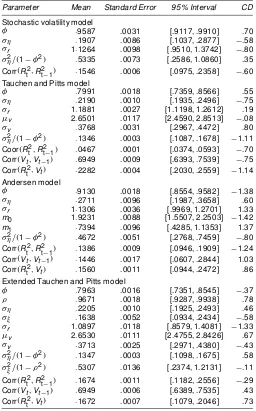
Estimation results are summarized in Tables 30and 40, which should replace Tables 3 and 4 of Watanabe (2000). (The revised version of Fig. 1 is omitted.) The reported convergencediagnos-tic statisconvergencediagnos-tics suggest that all chains are stationary. The posterior mean ofÁin the Tauchen and Pitts (1983) model shown in Ta-ble 30is:7991, which is much smaller than that of:9587 in the stochastic volatility model and close to the :801 obtained by
Table 30. Estimation Results
Parameter Mean Standard Error 95% Interval CD
Stochastic volatility model
Extended Tauchen and Pitts model
Á :7963 .0016 [.7351, .8545] ¡.37
NOTE: The rst 1,000 draws are discarded, and the next 10,000 are used for calculating the posterior means, the standard errors of the posterior means, 95% interval, and the convergence diagnostic (CD) statistics proposed by Geweke (1992). The posterior means are computed by averaging the simulated draws. The standard errors of the posterior means are computed using a Parzen window with a bandwidth of 1,000. The 95% intervals are calculated using the 2.5th and 97.5th percentiles of the simulated draws. The sample autocorrelation coefcient of squared returns is .1837. The sample autocorrelation coefcient of trading volume is .6999. The sample correlation coefcient between squared returns and trading volume is .2473.
Liesenfeld and Richard (2002). The posterior mean ofÁin the Andersen (1996) model also drops to:9130.
The main results of Watanabe (2000) are: (1) the Tauchen and Pitts (1983) model cannot account for the persistence in squared returns, whereas the Andersen (1996) model cannot ac-count for the persistence in trading volume, and (2) the Tauchen and Pitts (1983) model yields too-narrow Bayesian condence intervals of the out-of-sample squared returns. These results are still found to hold true.
ACKNOWLEDGMENTS
The author would like to thank Roman Liesenfeld and Jean-Francois Richard for useful comments on Watanabe (2000). Without their comments, he could not have found an error in the multimove sampler. Thanks are also due to the associate
580 Journal of Business & Economic Statistics, October 2003
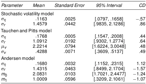
Table 40. Estimation Results WhenÁD1
Parameter Mean Standard Error 95% Interval CD
Stochastic volatility model
¾´ :1163 .0025 [.0797, .1658] ¡.57
¾r 1:4579 .0442 [.9835, 2.1286] .86
Tauchen and Pitts model
¾´ :1768 .0005 [.1547, .2008] .44
¾r 1:0912 .0192 [.9302, 1.2774] .64
¹v 2:2214 .0794 [1.6224, 3.0048] .48
¾v :4288 .0071 [.3609, .5137] .49
Andersen model
¾´ :1680 .0032 [.1152, .2315] 1.12
¾r 1:4315 .0463 [.8499, 2.1704] ¡1.57 m0 2:0831 .0103 [1.7021, 2.4477] ¡1.24 m1 1:0009 .0596 [.3209, 2.1061] ¡1.07
NOTE: The rst 2,000 draws are discarded, and the next 10,000 are used for calculating the posterior means, the standard errors of the posterior means, 95% interval, and the convergence diagnostic (CD) statistics proposed by Geweke (1992). The posterior means are computed by averaging the simulated draws. The standard errors of the posterior means are computed using a Parzen window with a bandwidth of 1,000. The 95% intervals are calculated using the 2.5th and 97.5th percentiles of the simulated draws.
editor Chris Lamoureux for helpful comments. Any remaining errors are the author’s alone.
[Received January 2003. Revised May 2003.]
REFERENCES
Andersen, T. G. (1996), “Return Volatility and Trading Volume in Financial Markets: An Information Flow Interpretation of Stochastic Volatility,” Jour-nal of Finance, 51, 169–204.
Chib, S., and Greenberg, E. (1995), “Understanding the Metropolis–Hastings Algorithm,”The American Statistician, 49, 327–335.
de Jong, P., and Shephard, N. (1995), “The Simulation Smoother for Time Se-ries Models,”Biometrika, 82, 339–350.
Geweke, J. (1992), “Evaluating the Accuracy of Sampling-Based Approaches to the Calculation of Posterior Moments,” in Bayesian Statistics 4, eds. J. M. Bernardo, J. O. Berger, A. P. Dawid, and A. F. M. Smith, Oxford, U.K.: Oxford University Press, pp. 169–193.
(2001), “Getting It Right: Checking for Errors in Likelihood-Based Inference,” working paper, University of Iowa.
Jacquier, E., Polson, N. G., and Rossi, P. E. (1994), “Bayesian Analysis of Stochastic Volatility Models” (with discussion),Journal of Business & Eco-nomic Statistics, 12, 371–417.
Liesenfeld, R. (1998), “Dynamic Bivariate Mixture Models: Modeling the Be-havior of Prices and Trading Volume,”Journal of Business & Economic Sta-tistics, 16, 101–109.
Liesenfeld, R., and Richard J. F. (2002), “The Estimation of Dynamic Bivariate Mixture Models: Comments on Watanabe (2000),” unpublished manuscript, Eberhard-Karls-Universität, Dept. of Economics.
Richard, J. F. (1998), “Efcient High-Dimensional Monte Carlo Importance Sampling,” unpublished manuscript, University of Pittsburg, Dept. of Eco-nomics.
Richard, J. F., and Zhang, W. (1996), “Econometric Modeling of U.K. House Prices Using Accelerated Importance Sampling,”The Oxford Bulletin of Eco-nomics and Statistics, 58, 601–613.
(1997), “Accelerated Monte Carlo Integration: An Application to Dy-namic Latent Variable Models,” inSimulation-Based Inference in Economet-rics: Methods and Application, eds. R. Mariano, M. Weeks, and T. Schuer-mann, Cambridge, U.K.: Cambridge University Press.
Shephard, N., and Pitt, M. K. (1997), “Likelihood Analysis of Non-Gaussian Measurement Time Series,”Biometrika, 84, 653–667.
Tauchen, G. E., and Pitts, M. (1983), “The Price Variability–Volume Relation-ship on Speculative Markets,”Econometrica, 51, 485–505.
Tierney, L. (1994), “Markov Chains for Exploring Posterior Distributions” (with discussion),The Annals of Statistics, 21, 1701–1762.
Watanabe, T. (2000), “Bayesian Analysis of Dynamic Bivariate Mixture Mod-els: Can They Explain the Behavior of Returns and Trading Volume?,” Jour-nal of Business & Economic Statistics, 18, 199–210.
Watanabe, T., and Omori, Y. (2001), “Multi-Move Sampler for Estimating Non-Gaussian Time Series Models: Comments on Shephard and Pitt (1997),” Re-search Paper 25, Tokyo Metropolitan University, Faculty of Economics.