Full Terms & Conditions of access and use can be found at
http://www.tandfonline.com/action/journalInformation?journalCode=ubes20
Download by: [Universitas Maritim Raja Ali Haji] Date: 11 January 2016, At: 23:20
Journal of Business & Economic Statistics
ISSN: 0735-0015 (Print) 1537-2707 (Online) Journal homepage: http://www.tandfonline.com/loi/ubes20
Data-Driven Bandwidth Selection for
Nonstationary Semiparametric Models
Yiguo Sun & Qi Li
To cite this article: Yiguo Sun & Qi Li (2011) Data-Driven Bandwidth Selection for Nonstationary Semiparametric Models, Journal of Business & Economic Statistics, 29:4, 541-551, DOI: 10.1198/jbes.2011.09159
To link to this article: http://dx.doi.org/10.1198/jbes.2011.09159
Published online: 24 Jan 2012.
Submit your article to this journal
Article views: 227
View related articles
Data-Driven Bandwidth Selection for
Nonstationary Semiparametric Models
Yiguo S
UNDepartment of Economics, University of Guelph, Guelph, ON, Canada N1G 2W1 (yisun@uoguelph.ca)
Qi L
IDepartment of Economics, Texas A&M University, College Station, TX 77843-4228 (qi@econmail.tamu.edu)
This article extends the asymptotic results of the traditional least squares cross-validatory (CV) bandwidth selection method to semiparametric regression models with nonstationary data. Two main findings are that (a) the CV-selected bandwidth is stochastic even asymptotically and (b) the selected bandwidth based on the local constant method converges to 0 at a different speed than that based on the local linear method. Both findings are in sharp contrast to existing results when working with weakly dependent or independent data. Monte Carlo simulations confirm our theoretical results and show that the automatic data-driven method works well.
KEY WORDS: Integrated time series; Local constant; Local linear; Semiparametric varying-coefficient model.
1. INTRODUCTION
It is well known that the capability of selecting the opti-mal smoothing parameter is crucial to the application of non-parametric estimation techniques. For independent and weakly dependent data, plug-in methods and (generalized) cross-validation (CV) methods have been incorporated into many popular software packages, and the corresponding asymptotic theory has been well developed (e.g.,Härdle and Marron 1985). However, to the best of our knowledge, no asymptotic analy-sis exists for studying the performance of bandwidth selection methods when integrated time series data are involved, even though nonparametric/semiparametric estimation of regression models with integrated processes has recently attracted much attention among econometricians and statisticians (see, e.g.,
Juhl 2005;Karlsen, Myklebust, and Tjostheim 2007; Cai, Li, and Park 2009;Phillips 2009;Wang and Phillips 2009a,2009b;
Xiao 2009). This article aims to fill this gap.
We focus on a particular type of semiparametric model, the semiparametric varying-coefficient model with integrated re-gressors. Cai, Li, and Park (2009) and Xiao (2009) derived the asymptotic properties of kernel estimators for this model, but used ad hoc methods for selecting the smoothing parame-ter. In this article we suggest using the least squares CV (LS– CV) method to choose the smoothing parameter and examine the asymptotic properties of this data-driven method–selected smoothing parameter. We consider the following semiparamet-ric model:
Yt=XtTβ(Zt)+ut, 1≤t≤n, (1.1)
whereYt,Zt, andutare scalars,Ztandutare stationary variables
withE(ut|Zt)=0 for allt,Xtis ap×1 vector containing some
nonstationary components, andβ(Zt)is ap×1 vector of
un-specified smooth functions. In situations where all of the vari-ables are weakly dependent or iid, model (1.1) was considered byChen and Tsay(1993), Cai, Fan, and Yao (2000), andZhou and Liang(2009), among others. When Zt=t, Equation (1.1)
was considered by Robinson (1989) and Cai (2007). Model
(1.1) adds extra flexibility to a linear cointegrating regression model by allowing the cointegrating vector to be smooth func-tions of some stationary variables. If some or all of the coeffi-cient functions are constant, then model (1.1) becomes a par-tially linear or linear cointegrating regression model. Thus our asymptotic result also covers the popular partially linear model; see Section2.4for a more detailed discussion of this.
To estimate the unknown coefficient curve β(·) in model (1.1), we apply both the local constant and the local linear re-gression approaches. The local constant (LC) estimator ofβ(z)
is given by
ˆ
β(z)=
n
t=1
XtXtTKh,tz
−1 n
t=1
XtYtKh,tz, (1.2)
whereKh,tz=h−1K(Zth−z),K(·)is a kernel function, andh is
the smoothing parameter. The local linear estimator of β(z), along with the estimator of its derivative function β(1)(z)=
dβ(z)/dz, is given by β(ˆ z)
ˆ
β(1)(z)
=
n
t=1 Kh,tz
1 Zt−z Zt−z (Zt−z)2
⊗(XtXtT)
−1
×
n
t=1 Kh,tz
Xt Xt(Zt−z)
Yt, (1.3)
where “⊗” denotes the Kronecker product.
In this article we are interested in studying the asymptotic properties of the LS–CV–selected bandwidth for both the local constant and the local linear estimator defined earlier whenXt
contains integrated covariates. We show that the CV-selected bandwidth is stochastic even asymptotically, and that the CV-selected bandwidth for the local constant estimator and the local
© 2011American Statistical Association
Journal of Business & Economic Statistics October 2011, Vol. 29, No. 4
DOI:10.1198/jbes.2011.09159
541
linear estimator converge to 0 at different speeds. Both findings are in sharp contrast to the existing results obtained for indepen-dent and weakly depenindepen-dent data cases. We show that the local linear estimation method has smaller estimated mean squared error than the local constant estimation method. We also show that the asymptotic properties of the CV-selected bandwidth re-main unchanged when theI(1)regressor is correlated with the error termut, provided that the correlation between theI(1)
re-gressor and the error termutis not overly persistent [see
Equa-tion (2.7) for the detailed condition].
To simplify notation/proofs without affecting the essence of our results, we give our theories and proofs for scalar cases; that is,Xtis a scalarI(1)variable in Section2, andXt=(Xt1,Xt2)T is a 2×1 vector, withXt1anI(0)variable andXt2anI(1) vari-able in Section3. Allowing higher dimensions inXt will only
make the mathematical representation of the asymptotic results more complicated without providing any additional insight into the problem.
The rest of the article is organized as follows. Section2 de-scribes the cross-validation method and derives asymptotic re-sults whenXt in model (1.1) is anI(1)variable. Section3
pro-vides asymptotic analysis whenXt=(Xt1,Xt2)T, whereXt1 is anI(0)variable andXt2is anI(1)variable. Section4presents Monte Carlo simulations. We relegate all mathematical proofs to two appendices.
2. CROSS–VALIDATION METHOD WITH ANI(1) COVARIATE
2.1 The CV Function and Regularity Conditions
Lethˆ be the data-driven bandwidth selected to minimize the following LS–CV function:
CV(h)= 1
n2 n
t=1
[Yt−XtTβˆ−t(Zt)]2M(Zt), (2.1)
where 0≤M(·)≤1 is a nonnegative weight function that trims out observations near the boundary of the support of Zt and
ˆ
β−t(Zt)is the leave-one-out local constant or local linear
es-timator ofβ(Zt)defined in Section1. Apparently, scaling the
CV function byn−2rather than the conventional choice ofn−1
is introduced purely for theoretical reasons, and this does not affect the value of the selected bandwidth minimizing (2.1). With a scale ofn−2,CV(h)asymptotically has the same order as
(β(ˆ z)−β(z))2M(z)dz, because sup1≤t≤nXt2/n=Op(1).
Thus,CV(h)with the scale ofn−2, can be roughly viewed as a weighted version of the average squared error of the nonpara-metric estimatorβ(ˆ ·); we provide a more detailed discussion of this point later.
To simplify notation, we write βt=β(Zt),βˆ−t= ˆβ−t(Zt),
andMt=M(Zt)for allt. Substituting (1.1) into (2.1) gives CV(h)= 1
n2
t
[XtT(βt− ˆβ−t)]2Mt
+n22
t
utXTt(βt− ˆβ−t)Mt+
1
n2
t
u2tMt, (2.2)
where the last term does not depend on h. Thus minimiz-ingCV(h)over h is equivalent to minimizingCV0(h), where CV0(h)consists of the first two terms ofCV(h),
CV0(h) def
=n−2 t
[XTt(βt− ˆβ−t)]2Mt
+2n−2 t
utXtT(βt− ˆβ−t)Mt
=CV0,1+2CV0,2, (2.3) where the definitions of CV0,1 and CV0,2 should be appar-ent. In Appendix A we show that CV0,1 is the leading term of CV0(h). With CV0,1=n−1t[X
T t
√
n(βt− ˆβ−t)] 2M
t, and by
supt|Xt|/√n=Op(1), we would expectCV0,1to have the same order as
(β(z)− ˆβ(z))2M(z)dz. We make the following assumptions:
A1 {Zt}is a strictlyβ-mixing stationary sequence of size
−(2+δ′)/δ′for some 0< δ′< δ <1, andE|Zt|2+δ< M<∞. Define M= {z∈R:M(z) >0}[the support of the weight functionM(·)]. We require thatMbe a compact subset ofR. Letf(z)be the pdf ofZt. Then f(z)has bounded derivatives (uniformly inz∈M) up to the fourth order, and infz∈Mf(z) >0.
A2 β(z)is not a linear function and is continuously differ-entiable up to the fourth order overz∈M.
A3 LetFnt=σ (Xi+1,Zi+1,ui:i≤t)be the smallest sigma
field containing the past history of{(Xi+1,Zi+1,ui)}ti=0.
Here(ut,Fnt)is a martingale difference sequence with E(u2t|Fn,t−1)=σu2 < ∞ for all t and suptE(|ut|q| Fn,t−1) <∞ for some q>2. In addition, the error termsutare independent of{(Xt,Zt)}nt=1.
A4 The kernel function K(·) is a symmetric (around 0) bounded probability density function on the interval
[−1,1].
A5 nh3(lnn)2→0, h[ln(n)]4→0, and n1−ǫh→ ∞ for some (arbitrarily) smallǫ >0, asn→ ∞.
A6 Letvt=Xt=Xt−Xt−1andηt(z)=et(z)−E(et(z)),
whereet(z)=(β(Zt)−β(z))Kh,tz and Kh,tz=h−1× K((Zt−z)/h). The partial sums of the vector process
(vt, ηt,utKh,tz)follow a multivariate invariance
princi-ple,
Bn,x(r)
Bn,β,z(r) Bn,u,z(r)
=
⎡
⎢ ⎣
n−1/2[nr]
t=1vt
(nh)−1/2[nr]
t=1ηt(z)
√
h/n[nr]
t=1utKh,tz
⎤
⎥ ⎦
⇒
B
x(r) Bβ,z(r) Bu,z(r)
def
=BM(0, ), (2.4)
where BM(0, ) denotes a Brownian motion with mean 0 and finite nonsingular variance–covariance ma-trix. Here[a]is the integer part ofaandr∈ [0,1]. A6* On a suitable probability space, there exists a vector
Brownian process, BM(0, ), with mean 0 and finite
nonsingular variance–covariance matrix such that
(i) sup
r∈[0,1]|
Bn,x(r)−Bx(r)| =op(1),
sup 1≤t≤n|
Xt| =O
√
nln lnn
almost surely; (2.5)
(ii) sup
z∈M sup
r∈[0,1]
Bn,β,z(r) Bn,u,z(r)
−
Bβ,z(r) Bu,z(r)
=op(1). (2.6)
Assumptions A1 and A2 impose a β-mixing weak depen-dence condition onZtand some moments and smoothness
con-ditions onf(z)andβ(z). Assumption A3 assumes thatut is a
martingale difference process independent of{(Xt,Zt)}nt=1, and this assumption significantly simplifies our proofs. Later we discuss how to relax Assumption A3 in two ways: (a) allow-ing forutto be a stationary mixing process in Assumption A3′,
which relaxes the martingale difference assumption, and (b) al-lowing ut to be correlated with (Xt,Zt) in Assumption A3′′,
which removes the independence assumption. Assumptions A4 and A5 impose mild conditions on the kernel function and the bandwidthh. The kernel function with a compact support is not essential and can be removed at the cost of a lengthy proof. As-sumption A5 implies thatnh/[ln(n)]d→ ∞ for any constant
d>0.
In Assumption A6, the weak convergence of the vector of the partial sums holds under some standard regularity conditions, such as strong mixing of{(vt,Zt,ut)}with some moment
con-ditions. Assumption A6* imposes strong convergence results on the partial sums. Similar conditions were used by Wang and Phillips (2009a). Note that Equation (2.6) in Assumption A6* requires a uniform convergence result of(Bn,β,z(r),Bn,u,z(r))
overz∈M. Equation (2.5) is a result of the functional law of the iterated logarithm (seeRio 1995).
Under Assumptions A1–A3,Bx(r),Bβ,z(r), andBu,z(r)are
independent of one another because the asymptotic covariances between each pair of the partial sums Bnx(r), Bn,u,z(·), and Bn,β,z(·)are 0, with the variances ofBβ,z(r)andBu,z(r)given
by σ12(z) = limn→∞var([tnr=1](nh)− 1/2η
1,nt(z)) = ν2(K) ×
[β(1)(z)]2f(z)andσ22(z)=limn→∞var(√h/nt[=nr1]utKh,tz)=
σu2v0(K)f(z), respectively, with νj(K)=ujK2(u)du. In
Sec-tion 2.3, we show that the independence between Bx(r) and Bu,z(r)also holds under the “weaker” Assumption A3′′. Write Wβ(r) = Bβ,z(r)/σ1(z) and Wu(r) = Bu,z(r)/σ2(z). Then
(Wβ(r),Wu(r)) is a bivariate standard Brownian motion
vec-tor independent of the stochastic processBx(r).
The foregoing assumptions exclude the cases where the er-ror term ut is serially correlated and the integrated variables
are endogenous. These assumptions are imposed to simplify the proofs and can be replaced by the weaker Assumption A3′, or by Assumption A3′′.
A3′ Same as Assumption A3 with this exception: Instead of assuming thatut is a martingale difference process, ut
is a strictly stationaryα-mixing process with mean 0, variance σu2<∞, and mixing coefficientsα(τ )≡ατ
satisfyingατ =O(τ−p)for some p> δ1/(δ1−2)and
δ1>2. Also,E(|ut|δ1)is finite.
The following (endogeneity) assumption is motived by Saikkonen’s (1991) idea. Assumption 2 of Wang and Phillips
(2009b) is in a similar spirit but more general than ours, be-cause their assumption 2 allows a potential nonlinear relation betweenutandvs.
A3′′ The following representation ofut allowsXt to be
en-dogenous:
ut= k0
j=−k0
αjvt−j+εt, (2.7)
where{εt}nt=1is independent of {(vt,Zt)}nt=1 andk0 is a nonnegative integer. In addition, ωt=(εt,vt)T is a
strictly stationary β-mixing process with mean 0 and mixing coefficientsβ(τ )≡βτ satisfyingβτ=O(τ−q)
for some q>2(1+δ′)/δ′ and 0< δ′< δ <1, andωt
has a finite fourth moment. In addition, lim var(n−1/2×
n
t=1ωt)is a finite, positive definite matrix. Moreover, E(u2t|zt=z)is continuously differentiable up to the
sec-ond order overz∈M.
Here we mainly use Assumption A3 (along with other as-sumptions) to prove the main results of the article. In supple-mental Appendix B (available from the authors on request), we briefly discuss how the proofs can be modified so that our re-sults remain valid even when Assumption A3 is replaced by Assumption A3′or by Assumption A3′′.
2.2 Main Results
In this section we present the asymptotic results of hˆ min-imizing (2.1) where the leave-one-out estimator can be either the local constant or the local linear estimator. The results are given in Theorem2.1for the local constant estimation case and in Theorem2.2for the local linear estimation case.
Theorem 2.1. Let hˆlc denote the cross-validation–selected
bandwidth based on the local constant estimation method. Un-der Assumptions A1–A5 and A6*, and assuming that β(z)is not a constant function, we have
(i) CV(h)− 1
n2 n
t=1
u2tM(zt)−CVlc,L(h)=op(h/n+(n2h)−1),
(2.8)
where
CVlc,L(h)= h nν2(K)B
−1 x,(2)
M(z)β(1)(z)2dz
ζβ,22
+n12hν0(K)σu2
M(z)dz B−x,(12)ζu,21, (2.9)
Bx,(2)=01Bx2(r)dr,ζi,j=01Bjx(r)dWi(r)fori=β,uandj=
1,2;
(ii) √nhˆlc−σu
ζu,21ν0(K)M(z)dz
ζβ,22ν2(K)
M(z)[β(1)(z)]2dz p
→0.
(2.10)
The proof of Theorem 2.1 is given in Appendix A. The-orem 2.1(i) states that, apart from a term (n−2
tu2tMt) that
does not depend onh,CVlc,L(h)is the leading term ofCV(h).
This leading term consists of two parts: theOp(h/n)term
cor-responding to the leading bias term, and the(n2h)−1term from the leading variance term. The selected bandwidth balances these two terms, and we obtainhˆlc=Op(n−1/2), as stated in
Theorem2.1(ii).
A fundamental difference between the result presented in Theorem2.1and previously reported results (when dealing with independent or weakly dependent data) is that the “optimal” bandwidth is stochastic even asymptotically. More specifically, let the CV-selected bandwidth behˆlc= ˆcn−α. With weakly
de-pendent or indede-pendent data, it is well known thatα=1/5 and
ˆ
c→p copt, wherecopt>0 is a nonstochastic (optimal) constant
so thathˆlc/hopt p
→1, andhopt=coptn−1/5is the nonstochastic
benchmark (optimal) bandwidth (see Härdle, Hall, and Marron
1992). In contrast, when Xt is anI(1) process, Theorem 2.1
states that α=1/2, and that cˆ does not converge to a non-stochastic constant, but insteadcˆhas a well-defined nondegen-erate limiting distribution. Simulation results in Section4 con-firm the theoretical results of Theorem2.1. There we show that, as the sample sizenincreases,hˆlcshrinks to 0, whereascˆhas a
stable nondegenerate distribution. The next theorem describes the asymptotic behavior for the LL–CV–selected bandwidth.
Theorem 2.2. Let hˆll denote the CV-selected bandwidth
based on the local linear estimation method. Under Assump-tions A1–A5 and A6*, we have
(i) CV(h)−n−2 n
t=1
u2tMt−CVll,L(h)=op(h4+(n2h)−1),
(2.11)
where
CVll,L(h)=(1/4)h4Bx,(2)κ22E
βt(2)
2
Mt
+(n2h)−1ν0(K)σu2B− 1 x,(2)ζ
2 u,1
M(z)dz, (2.12)
κ2=v2K(v)dv, andβt(2)=d2β(z)/dz2|z=Zt;
(ii) n2/5hˆll−
4σ2
uν0(K)M(z)dzζu,21 B2x,(2)κ22E[(βt(2))2Mt]
1/5
p
→0. (2.13)
The proof of Theorem 2.2 is given in supplemental Ap-pendix B, where we show thatCVll,L(h)=Op(h4+(n2h)−1).
TheOp(h4)term corresponds to the leading bias term, and the Op(n2h)−1 term is the leading variance term. The “optimal” h balancing the two terms has an order ofn−2/5. We explain why the leading bias term from the LL estimation method dif-fers from that obtained from the LC estimation method in Sec-tion2.3.
Theorems 2.1 and2.2 imply that CVlc,L(hˆlc)=Op(n−3/2)
and CVll,L(hˆll)=Op(n−8/5), respectively. Thus the LC–CV
method gives stochastically a larger average squared error than that obtained from the LL–CV method, indicating that the LL– CV method dominates the LC–CV method. This is in sharp contrast to the existing results obtained for independent or
weakly dependent data, because it is well known that for inde-pendent or weakly deinde-pendent data cases, the CV functions for the local constant and the local linear methods have the same rate of convergence.
Note that the result of Theorem2.1requires thatβ(z)be a nonconstant function, and that Theorem2.2assumes thatβ(z)
is nonlinear inz. Here we briefly comment on what happens if these assumptions are violated. First, if Pr{β(Zt)=c} =1 for
some constantc, then the true model reduces to a linear coin-tegration model. Ideally, one would like to select a sufficiently largehin this case, because whenh= +∞,β(ˆ z)becomes the least squares estimator of the constant parameterc. However, it can be shown that neitherhˆlcnorhˆllwill converge∞in this
case. Moreover,hwill not converge to 0, so our Theorems2.1
and2.2do not cover the case whereβ(·)is a constant function. We conjecture that the CV-selected bandwidth has a tendency to take large positive values but will not diverge to infinity even asn→ ∞. Simulations reported in Section4support our con-jecture. The asymptotic behavior of the CV-selected bandwidth when the true regression model is linear (β is a constant) is quite complex, and it is beyond our present capabilities to de-rive the asymptotic distribution of the CV-selected bandwidth in this case.
Next, if Pr{β(Zt)=a+bZt} =1, or β(z)is a linear
func-tion inz, then it can be shown that in this case, Theorem2.1
still holds true so thathˆlc=Op(n−1/2)(hˆlcstill converges to 0),
whereashˆllconverges to neither 0 nor∞. In Section 4 we use
simulations to investigate the behavior ofhˆcv when β(z)=a
andβ(z)=a+bz. We also examine a spurious regression case whereβ(z)≡0 and ut is an I(1)process. The theoretical
in-vestigation of hˆcv under a spurious regression model is quite
complicated and is beyond the scope of this article.
2.3 Endogenous Regressor Case
For a linear cointegration model, it is well known that when
Xtandutare correlated, the ordinary least squares (OLS)
esti-mator of the cointegrating coefficient is stilln-consistent but has an additional bias term of ordern−1 (seePhillips and Hansen 1990;Phillips 1995). Recently, Wang and Phillips (2009b, the-orem 3.2) considered a nonparametric cointegration model and showed that the asymptotic analysis remains unchanged even whenXt is correlated withut, provided that the correlation is
not overly persistent. However, Wang and Phillips’ framework is quite different from the semiparametric model that we con-sider here, because in their model, the nonstationary variable enters the model nonparametrically, whereas in our semipara-metric model, the nonparasemipara-metric componentZt is a stationary
variable. To the best of our knowledge, in the framework of a semiparametric varying-coefficient model withI(1)regressors, the endogeneity issue has not been addressed. A priori, it is not clear whether an endogenous regressor will lead to a nonneg-ligible bias term. In this section we show that the asymptotic distribution ofβ(ˆ z)remains unchanged whenXt is correlated
withut under some standard regularity conditions. For
exposi-tional simplicity, we consider only the local constant estimator in this section; a similar result can be shown to hold true for the local linear estimator.
LetKh,tz=h−1K((Zt−z)/h). Then the local constant
esti-lowingXtandutto be correlated may affect the asymptotic
be-havior only ofA3n, because other terms do not depend onut. We
show that the asymptotic behavior ofA3n remains unchanged
when Assumption A3 is replaced by Assumption A3′′. There-fore, our result remains the same even whenXt is correlated
withut.
UsingXt=ts=1vt, we haveA3n=n−2nt=2Xt−1utKh,tz+ n−2n
t=1vtutKh,tz, where the stochastic property of vt is
de-scribed in Assumption A3′′. If ut is a martingale difference
sequence as defined in Assumption A3, or ifXt is strictly
ex-ogenous withE(ut|Zt)=0, we haveE(A3n)=0. However,
al-lowing Xt to be endogenous and ut to be serially correlated
generally leads to E(A3n)=0. Assumption A3′′ ensures that
supz∈Mn−1nt=1|vtut|Kh,tz=Op(1), and applying
Assump-tion A6 and theorem 4.1 of De Jong and Davidson (2000) gives
n√hA3n= that has a finite second moment. By Assumptions A1 and A3′′,
{(Zt,vt,ut)}nt=1is aβ-mixing process. Thus, applying lemma 1
ofYoshihara(1976), we obtain
|n| ≤
Therefore, the bias term due to the correlation between
Xt and ut is asymptotically negligible, which differs from
the linear regression model case. Replacing Kh,tz by 1 in
(2.14), we obtain the OLS estimator of β. It is easy to see that for a linear cointegration model, the bias term is 0
def
=0, because our bias term has an additional factor√hKh,tz
andE[√hKh,tz] =O(
√
h)=o(1).
We use the foregoing decomposition to provide an intuitive explanation of Theorem2.1as to whyCVlc,L(h)=Op(h/n+
Here the notation Oe(an)means an exact probability order of Op(an), but is notop(an).
Next considerA2n. By adding/subtracting terms, we rewrite A2n=A2n,1+A2n,2, where
us that the order of A2n,2 is determined by the variance part of et(z) as ηt(z)has mean 0. With weakly dependent data, it
is well known that the mean part ofet(z)dominates the
vari-ance part of et(z). However, if the local constant estimation
method is used to analyze integrated time series, then the vari-ance part of et(z) dominates the mean part of et(z). To see
this, we square each term to get rid of the square root ex-pressions, which givesA22n,1=Op(h4),A22n,2=Op(h/n), and A23n=Op((n2h)−1). These results imply that A22n,2+A23n= Op(h/n+(n2h)−1)has a stochastic order larger than that of A22n,1=Op(h4).
The foregoing analysis also provides an explanation as to why the leading term of the CV function, CVlc,L(h),
con-tains two terms of orders Op(h/n) and Op((n2h)−1), which
are related to the variances of et(z) and utKh,tz, respectively.
The Op(h4)term corresponding to the squared mean ofet(z)
is asymptotically negligible. However, if the local linear esti-mation method is used instead of the local constant method,
β(Zt)−β(Zs)must be replaced byR(Zt,Zs) def
=β(Zt)−β(Zs)−
β(1)(Zt)(Zt−Zs). In this case the two leading terms,Op(h4)
and Op((n2h)−1) [of CVll,L(h)], correspond to the (squared)
mean ofR(Zt,Zs)Kh,tzand the variance ofutKh,tz, whereas the
term related to the variance of R(Zt,Zs)Kh,tz, which has order Op(h4/n)(this term differs from the LC case), is asymptotically
negligible. Therefore, the reason for the different convergence rates ofCVlc(h)andCVll(h)is that, unlike in the weakly
de-pendent data case, the LC and the LL estimator have different stochastic orders inAn2.
It can be shown that the results of Theorems2.1and2.2hold true whenXtandutare correlated, but the proofs will be lengthy
and tedious and will provide no additional insight into the prob-lem. Thus to save space, we do not pursue proofs for Theo-rems2.1and2.2for the endogenousXt case. In Section4we
report Monte Carlo simulations that allow Xt to be correlated
withut. The simulation results reported there support the
fore-going theoretical analysis and show that the estimation results are virtually unaffected whether or notXtandutare correlated.
2.4 A Partially Linear Varying-Coefficient Model
In this section we consider the CV selection of the band-widthhwhen estimating the following partially linear varying-coefficient model:
Yt=STtγ+Xtβ(Zt)+ut, (2.19)
where St is a (d−1)×1 vector of I(1)variables, and γ is
a(d−1)×1 vector of constant parameters. For expositional simplicity, we assume thatXtis a scalarI(1)variable. Note that
the foregoing partially linear model is a special case of a general varying-coefficient modelYt=StTα(Zt)+Xtβ(Zt)+ut, where
the restriction thatα(z)≡γ, a vector of constant parameters, is imposed.
We propose using a profile least squares approach to esti-mateγ. First, we treatγ as if it were known and rewrite (2.19) asYt−STtγ =Xtβ(Zt)+ut. Then the local constant estimator
ofβ(Zt)is given by
˜
β(Zt)=
s
Xs2Kh,ts
−1
s
Xs(Ys−STsγ )Kh,ts
≡A2t−AT1tγ , (2.20)
whereA1t=(sXs2Kh,ts)−1sXsSsKh,tsandA2t=(sXs2× Kh,ts)−1sXsYsKh,ts. Note that β(˜ Zt)defined in (2.20) is
in-feasible, because it depends on the unknown parameterγ. We provide a feasible estimator forβ(Zt)in (2.23). Replacingβ(Zt)
byβ(˜ Zt)in (2.19) and rearranging terms, we obtain
Yt−XtA2t=(St−XtA1t)Tγ+ǫt, (2.21)
where ǫt ≡Yt −XtA2t−(St−XtA1t)Tγ. Applying the OLS
method to model (2.21) leads to
ˆ
γ=
t
(St−XtA1t)(St−XtA1t)T
−1
×
t
(St−XtA1t)(Yt−XtA2t). (2.22)
Replacingγwithγˆin (2.20), we obtain a feasible leave-one-out estimator ofβ(Zt)given by
ˆ
β−t(Zt)=
s=t X2sKh,st
−1
s=t
Xs(Ys−STsγ )ˆ Kh,st. (2.23)
It can be shown thatSTt(γ − ˆγ )has a stochastic order smaller thanXt(βt− ˆβ−t). Thus the leading term ofCVγˆ(h)=n−2×
n
t=1[Yt−StTγˆ−Xtβˆ−t(Zt)]2Mtis given byCVγ(h)=n−2×
n
t=1[Yt −STtγ −Xtβˆ−t(Zt)]2Mt. Obviously, CVγ(h) is the
same as CV(h) defined in (2.1). This is because if we de-fineY˜t=Yt−STtγ, then model (2.19) can be written asY˜t= Xtβ(Zt)+ut, which is identical to model (1.1). Thus the
re-sults of Theorem2.1remain valid for the partially linear model (2.19).
The foregoing discussion is based on the local constant esti-mation method. The local linear estiesti-mation method could be used as well. In this case, β(˜ z) in (2.20) is replaced by the local linear estimator, which is also linear inγ. The remain-ing estimation steps are similar to the local constant estimation case discussed earlier. The asymptotic behavior of the LS–CV– selectedhis the same as presented in Theorem2.2.
3. Xt CONTAINS BOTHI(0) ANDI(1) COMPONENTS
The results in Section2are obtained assuming thatXt
con-tains onlyI(1)components. This assumption simplifies our the-oretical analysis and makes it easier to see why the LC and LL estimation methods lead to different rates of convergence. How-ever, in practice, a cointegration model also may include an intercept term and some other stationary variables in addition to someI(1)regressors. Therefore, in this section we investi-gate the asymptotic behavior of the LS–CV–selected bandwidth whenXtcontains bothI(0)andI(1)components. Specifically,
we considerXt=(X1t,X2t)T withX1t andX2t beingI(0)and I(1)variables, respectively. We replace Assumption A6* by the following assumption:
B LetXt=(X1t,X2t)T, whereX2tsatisfies Assumption A6*
given in Section2andX1tis a strictly stationaryβ-mixing
sequence of size−(2+δ′)/δ′ for some 0< δ′< δ with
E(|X1t|2+δ) <M <∞. In addition, both E(X1t|Zt =z)
and E(X12t|Zt=z) are twice continuously differentiable
overz∈M.
Given that the local linear method has a smaller asymptotic MSE than the local constant method, we consider only the local linear estimation method in this section.
Theorem 3.1. Lethˆ denote the CV-selected bandwidth via the local linear method. Under Assumptions A1–A5 and B, we have
n2/5hˆ−c3n p
→0, (3.1)
wherec3nis a well-definedOe(1)random variable that is
deter-mined by (B1.2) and (B.13) in supplemental Appendix B.
Comparing the result of Theorem3.1with that of Cai, Li, and Park(2009), we see thathˆ (defined in Theorem3.1) is op-timal for estimatingβ2(·), the coefficient function associated with the integrated variable, because Cai, Li, and Park (2009)
showed that the optimalhfor estimatingβ1(·)should have an order ofn−1/5. The reason that the CV method selects an op-timalh for estimatingβ2(·)is becauseX2Ttβ2(Zt)is the
dom-inant component ofX1Ttβ1(Zt)+X2Ttβ2(Zt). Thus, to minimize
the CV function, one must choose anhthat is optimal for es-timatingβ2(·), the coefficient function of theI(1)covariate. In the next section, we examine a two-step estimation method as suggested by Cai, Li, and Park (2009) via Monte Carlo simula-tions, where after obtainingβˆ1(Zt)andβˆ2(Zt)in the first step,
we useYt−X2tβ(ˆ Zt)as the new dependent variable and
esti-mateβ1(Zt)using a new CV-selected smoothing parameter in
the second step. We show that this two-step method leads to improved estimation results forβ1(z).
4. MONTE CARLO SIMULATIONS
4.1 Case (a):Xt IsI(1)
We consider the following data-generating process (DGP):
Yt=Xtβ(Zt)+ut, Zt=0.5Zt−1+η3t, and ut=(η2t+θ η1t)/
1+θ2,
where Xt = Xt−1 + η1t, (η1t, η2t)T is iid N(0,I2), η3t is
iid Uniform[0,1], andX0=0. The data-generating mechanism for ut is the same as that of Wang and Phillips (2009b). It is
easy to show that corr(Xt,ut)=θ/
√
1+θ2. We take two val-ues forθ, θ=0 andθ =0.2, where the former case implies thatXtandutare independent of one another, whereas the
lat-ter case gives that corr(Xt,ut)=0.1961. Zt is a stationary
AR(1)process with the innovationη3ttaking values in[0,1].
We consider four different DGPs and index them by DGPi,j,
specifically,i=1 if θ =0, i=2 if θ =0.2, j=1 if β(z)=
1+z+2z2 whose value increases aszincreases, andj=2 if
β(z)=sin(3z), which is not monotone and has more curvature than the quadratic function. Comparing DGP1,jwith DGP2,jfor j=1 and 2, we aim to show thatXt is allowed to be correlated
withut as discussed in Section2.3. Comparing DGPi,1 with DGPi,2 for i=1 and 2, we examine how extra curvature of a coefficient function affects the finite-sample performance of our proposed CV method.
The sample sizes aren=100, 200, and 400. The number of simulations ism=1000. We report the square root of the av-erage squared error,RMSE=√AMSE, and the mean absolute bias,MABIAS, where for thelth simulation, we defineAMSEl= n−1n
t=1(β(zt)− ˆβl(zt))2 andMABIASl=n−1nt=1|β(zt)−
ˆ
βl(zt)|.
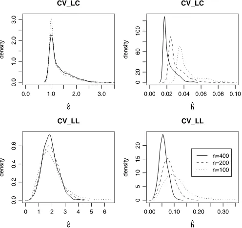
Figure1plots the kernel density functions of the CV-selected constantcˆand the bandwidthhˆ, wherehˆ= ˆcn−α withα=1/2 for the LC–CV method andα=2/5 for the LL–CV method. Figure1is obtained from DGP2,1, where the dotted line repre-sentsn=100, the dashed line representsn=200, and the solid line representsn=400. As predicted by Theorems2.1and2.2, we see that the CV-selected bandwidthhˆ becomes smaller as sample size increases, and thatcˆ does not converge to a con-stant as the estimated density function forcˆis rather stable for different sample sizes.
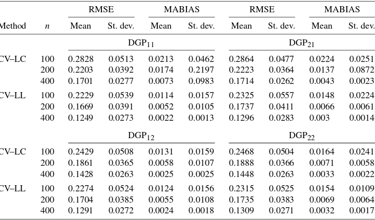
Table1 reports the mean and standard deviation (over the 1000 replications) of the RMSE and the MABIAS. Several in-teresting patterns are observed. First, the LL–CV method has
Figure 1. Kernel density estimate of CV-selected constant and bandwidth.
smaller (mean value of) RMSE and MABIAS compared with the LC–CV method. This is consistent with our theory, be-cause the LL–CV method has smaller asymptotic MSE than the LC–CV method, as shown in Theorems2.1and2.2. Second, the estimation efficiency gain of the LL–CV method over the LC–CV method is more pronounced for DGPi1than for DGPi2 fori=1,2 when the unknown curve has more curvature (i.e., more nonlinearity). Third, comparing the results of DGP1,jwith
DGP2,j for j=1 and 2 confirms our theoretical analysis
pre-sented in Section2.3that the CV method is valid even whenut
andXtare contemporaneously correlated.
To show how the CV-selected bandwidth behaves whenβ(·)
is constant, Table 2 reports the first quartile, median, mean, and third quartile of the CV-selected bandwidths, along with the RMSE and the MABIAS for the LC and LL kernel estima-tors, whereβ(z)≡1. The results forθ=0.2 andθ=0 are very similar, so we only report the results forθ=0. In addition, the bandwidth has an upper bound of five times the interquartile range of Zt (i.e., 9.45), because allowing the bandwidth to
in-crease further will improve the CV value only beyond the sixth decimal point. In this case, with a much larger selected band-width, the LC–CV method gives smaller RMSE and MABIAS than the LL–CV method. We also see that the median value of the LC–CV–selectedhis quite stable and does not seem to change asnincreases. This result is consistent with our earlier finding that whenβ(z)is a constant function, the CV method tends to choose a large value ofh, but the CV-selectedh will converge neither to∞nor to 0.
Table3reports the results whenXt andYt are two
indepen-dent random-walk processes without drift (a spurious regres-sion model). In this case theCV(h)objective function is quite flat, and the RMSE and the MBIASE do not change much even when thehchanges substantially, resulting a wide range of se-lectedhˆcv, as shown in Table3. Taken together, the results in
Tables2and3show that an unusually large LC–CV–selected
Table 1. The LC–CV vs. the LL–CV method whenXtis anI(1)variable
RMSE MABIAS RMSE MABIAS
Method n Mean St. dev. Mean St. dev. Mean St. dev. Mean St. dev.
DGP11 DGP21
CV–LC 100 0.2828 0.0513 0.0213 0.0462 0.2864 0.0477 0.0224 0.0251 200 0.2203 0.0392 0.0174 0.2197 0.2223 0.0364 0.0137 0.0872 400 0.1701 0.0277 0.0073 0.0983 0.1714 0.0262 0.0043 0.0023
CV–LL 100 0.2229 0.0539 0.0114 0.0157 0.2325 0.0557 0.0148 0.0224 200 0.1669 0.0391 0.0052 0.0105 0.1737 0.0411 0.0066 0.0061 400 0.1249 0.0273 0.0022 0.0013 0.1296 0.0283 0.003 0.0014
DGP12 DGP22
CV–LC 100 0.2429 0.0508 0.0131 0.0159 0.2468 0.0504 0.0164 0.0241 200 0.1861 0.0365 0.0058 0.0107 0.1888 0.0366 0.0071 0.0058 400 0.1428 0.0263 0.0025 0.0025 0.1448 0.0263 0.0033 0.0022
CV–LL 100 0.2274 0.0524 0.0124 0.0156 0.2315 0.0525 0.0154 0.0109 200 0.1704 0.0385 0.0055 0.0108 0.1735 0.0383 0.0069 0.0064 400 0.1291 0.0272 0.0024 0.0018 0.1309 0.0271 0.0032 0.0017
ˆ
hmay indicateβ(z)=c, a constant, or may suggest a spurious relationship betweenYt andXt. Further diagnostics are needed
to distinguish these two possibilities.
4.2 Case (b):Xt Contains BothI(0) andI(1) Variables
We consider the following DGP:
Yt=X1tβ1(Zt)+X2tβ2(Zt)+ut, (4.1)
where X2t =X2,t−1 +η1t, X1t = 1+0.5X1,t−1 +η4t with
η4t∼iid N(0,1), ut and Zt are generated as in Section 4.1,
β1(z)=1+z+2z2, andβ2(z)=sin(3z). We use DGP3 and DGP4to denote the cases whereθ=0 andθ=2, respectively. For DGP4, corr(X2t,ut)=0.8944, a rather high
contempora-neous correlation.
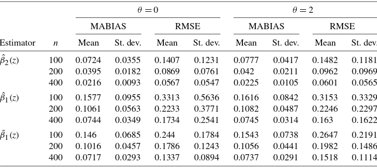
Table4presents simulation results for two estimators:β(ˆ ·), the LL–CV estimator using the LL–CV–selected bandwidthhˆ, andβ˜1(·), the two-step LL–CV estimator forβ1(·)in which we construct a new dependent variable Yt−X2tβˆ2(Zt)and
rees-timate β1(Zt) in the second stage, where βˆ2(Zt) is the
first-stage estimator of β2(Zt). We also selected a new bandwidth
via the LL–CV method in the second-stage estimation. We ob-serve the following. First, the coefficient curveβ2(·)associated with theI(1)variable is estimated more accurately than the co-efficient curveβ1(·)associated with theI(0)variable. Second,
the second-step estimation ofβ1(·)by the LL–CV method per-forms slightly better than the one-step estimation result ofβ1(·). Finally, Table4also indicates that we do not need the strictly exogenous assumption to validate the CV method.
APPENDIX A: PROOF OF THEOREM2.1
We use the notationAn=Bn+(s.o.)to denote thatAn=Bn+
terms are of smaller order thanBn. We denoteβt=β(zt),βt(j)=
β(j)(zt)=djβ(z)/dzj|z=zt, βˆ−t= ˆβ−t(zt), Kh,ts=h− 1K((z
t − zs)/h), ft=f(zt), Mt=M(zt), and s=t=ns=1,s=t. Also,
νj(K)=ujK(u)2du, κ2=u2K(u)du, c1n=n−2nt=1x2t, c2n=n−3nt=1xt4, and M= {z∈R:M(z) >0}.
Proof of Theorem2.1
By (1.2),βˆ−t=(s=tx2sKh,ts)−1s=txsYsKh,ts. Replacing Ysinβˆ−tbyYs=xsβs+us=xsβt+xs(βs−βt)+us, we obtain
ˆ
β−t=βt+ ˆAt−1(Bˆt+ ˆCt), (A.1)
whereAˆt=n−2s=tx2sKh,ts,Bˆt=n−2s=txs2(βs−βt)Kh,ts,
andCˆt=n−2s=txsusKh,ts.
Note that for cases of independent or weakly dependent data,
ˆ
At−1BˆtandAˆ−t 1Cˆtcorrespond to the bias and variance terms,
re-spectively. Therefore, for convenience we refer these two terms as bias and variance terms.
Table 2. The LC–CV vs. the LL–CV method whenXtis anI(1)variable andβ(z)≡1
ˆ
h RMSE MABIAS
Method n h0.25 h0.5 hmean h0.75 Mean St. dev. Mean St. dev.
CV–LC 100 8.0816 8.3528 8.3508 8.6341 0.0166 0.0168 0.0167 0.0166 200 8.3893 8.6057 8.5907 8.8187 0.008 0.0081 0.0082 0.0077 400 8.6099 8.7869 8.7863 8.9654 0.0037 0.0043 0.0041 0.0039 CV–LL 100 8.0823 8.3528 8.3588 8.634 0.0271 0.0214 0.0234 0.0186 200 8.3893 8.6057 8.5991 8.8187 0.0132 0.0104 0.0114 0.0088 400 8.6099 8.7869 8.7863 8.9654 0.0066 0.0055 0.0059 0.0046
Table 3. The LC–CV vs. the LL–CV method whenXtandYtare independent random walk processes
ˆ
h RMSE MABIAS
Method n h0.25 h0.5 hmean h0.75 Mean St. dev. Mean St. dev.
CV–LC 100 0.1355 0.3146 2.6275 7.8475 0.7366 0.6379 0.7156 0.6332 200 0.1347 0.2912 2.5119 7.8823 0.6990 0.6113 0.6863 0.6089 400 0.1589 0.3265 2.5747 6.3165 0.7014 0.6320 0.6941 0.6307
CV–LL 100 0.2393 0.7662 3.8878 8.2403 0.7538 0.6425 0.7233 0.6335 200 0.1943 0.5494 3.5212 8.4263 0.7157 0.6239 0.6923 0.6086 400 0.2195 0.7223 3.6277 8.5907 0.7133 0.6443 0.6981 0.6344
Substituting (A.1) intoCV0,1defined in (2.3), we obtain
CV0,1=n−2
t
(xtAˆ−t 1Bˆt)2Mt+n−2
t
(xtAˆ−t 1Cˆt)2Mt
+2n−2 t
xt2Aˆ−t 2BˆtCˆtMt
≡CV1+CV2+2CV3, (A.2) where the definitions ofCVj(j=1,2,3) should be apparent.
In LemmasA.2–A.4we show that
CV1=(h/n)Bx,(−12)ν2(K)E
Mtft−1
βt(1)2
×
1
0
B2x(r)dWβ(r)
2
+op(h/n+h3), (A.3)
CV2=
ν0(K)σu2 n2h B−
1 x,(2)
1
0
Bx(r)dWu(r)
2
M(z)dz
+op((n2h)−1), (A.4)
CV3=op(h/n), (A.5)
whereBx,(2)=01Bx(r)2dr andBx(r),Wβ(r), andWu(r)are
as defined in Section2.1. Under Assumptions A1–A3 and A6,
Wβ(r)andWu(r)are standard Brownian motions independent
of the stochastic processBx(r). Using similar arguments, it can
be shown that [CV0,2is as defined in (2.3)],
CV0,2=op(h/n)+Op
n2h1/2−1=op(h/n). (A.6)
Combining (A.3)–(A.6), we see that the leading term of
CV0(h)defined in (2.3) is given by CVlc,L(h)=(h/n)ν2(K)B−x,(12)
×EMtft−1
βt(1)
2
1
0
B2x(r)dWβ(r)
2
+ν0(K)σ
2 u n2h B−
1 x,(2)
1
0
Bx(r)dWu(r)
2
×
M(z)dz. (A.7)
Obviously,CVlc,L(h)is minimized at
h0=σun−1/2
ζu,21ν0(K)M(z)dz
ζβ,22ν2(K)M(z)(β(1)(z))2dz
=Oen−1/2, (A.8)
whereζij=01Bjx(r)dWi(r)fori=β,uandj=1,2.
The foregoing result can be extended to suph∈Hn|CV0(h)− CVlc,L(h)| =op(n−1/2), whereHn=(an−0.6,bn−0.4)for some a>0 andb>0. This completes the proof of Theorem2.1.
Lemma A.1. Under Assumptions A1, A2, A4, A5, and A6, we have
sup
zt∈M
| ˆAt− ˜μ1(zt)| =Op
( lnn)1/2 (nh)1/4
, (A.9)
whereμ˜1(z)=(n−2tx2t)f(z)≡c1nf(z).
Table 4. The LC–CV vs. the LL–CV method whenX1tis anI(0)variable andX2tis anI(1)variable
θ=0 θ=2
MABIAS RMSE MABIAS RMSE
Estimator n Mean St. dev. Mean St. dev. Mean St. dev. Mean St. dev.
ˆ
β2(z) 100 0.0724 0.0355 0.1407 0.1231 0.0777 0.0417 0.1482 0.1181
200 0.0395 0.0182 0.0869 0.0761 0.042 0.0211 0.0962 0.0969 400 0.0216 0.0093 0.0567 0.0547 0.0225 0.0105 0.0601 0.0565 ˆ
β1(z) 100 0.1577 0.0955 0.3313 0.5636 0.1616 0.0842 0.3153 0.3329
200 0.1061 0.0563 0.2233 0.3771 0.1082 0.0487 0.2246 0.2297 400 0.0744 0.0349 0.1734 0.2541 0.0745 0.0314 0.163 0.1622 ˜
β1(z) 100 0.146 0.0685 0.244 0.1784 0.1543 0.0738 0.2647 0.2191
200 0.1016 0.0457 0.1786 0.1243 0.1056 0.0441 0.1982 0.1486 400 0.0717 0.0293 0.1337 0.0894 0.0737 0.0291 0.1518 0.1114
Proof. By (2.5), we havet= ˆAt− ˜μ1(zt)=n−2s=tx2s×
tion A1, and applying the continuous mapping theorem, we haveMn(·)⇒B2x(·). We then have we also use the following results: by Assumption A6, we have
sup
In addition, in deriving the third line of Equation (A.10) we use theorem 6 ofHansen(2008):
Lemma A.2. Under Assumptions A1, A2, A4, A5, and A6*, (A.3) holds true.
Second, applying the same proof technique used in the proof of LemmaA.1, we can derive the stochastic order forω2t.
Specif-ically, we have (A.12). Also, applying theorem 2 ofHansen(2008) gives
sup
Finally, we considern3=n−2c−1n2
tx2tω22tMtft−2. By
As-sumption A6*, (2.6) with σ1(z)= |β(1)(z)|√ν2(K)f(z), we have 1
σ1(z)
√
nh
s x2
s
n[es(z)− E(es(z))] −
1
0B2x(r)dWβ(r) = op(1) uniformly over z∈ M. Also note that when c1n = n−2n
s=1x2s =Bx,(2)+op(1), whereBx,(2)=
1
0Bx(r)2dr, we have
n3=(h/n)ν2(K)B−x,(12)EMtft−1
βt(1)
2
1
0
B2x(r)dWβ(r)
2
+op(h/n). (A.19)
Combining (A.14), (A.18), and (A.19) completes the proof of LemmaA.2.
Lemma A.3. Under Assumptions A1–A6*, (A.4) holds true.
Proof. Lemma A.1 implies that the leading term of CV2, denoted byCV02, is obtained from CV2 by replacing Aˆt with
˜
μ1(zt). That is, CV02 =n−2
tx2tCˆt2/μ˜21(zt)Mt =n−2c−1n2 ×
tx2tCˆ2tf− 2
t Mt, where Cˆt =n−2s=txsusKh,ts. By
Assump-tion A6*, we haven√hCˆt=σu√v0(K)f(zt)01Bx(r)dWu(r)+ op(1). Therefore, we obtain
n2hCV20=σu2v0(K)c−1n1
1
0
Bx(r)dWu(r)
2
M(z)dz
+op(1). (A.20)
This completes the proof of LemmaA.3.
Lemma A.4. Under Assumptions A1–A6, (A.5) holds true.
Proof. By definition,CV3=n−4tx2tBˆtAˆ−t 2Mt×s=txs× usKh,ts. Assumption A3 implies that E(CV3)=0 and{ut}nt=1
are serially uncorrelated. Letting 3,n =E(CV23|{xt,zt}nt=1),
we have3,n=n−8σu2
t(x2tBˆtAˆ−t 2Mt)2s=tx2sKh,ts2 +n− 8×
σu2
t
t′=tx2tBˆtAˆt−2Mtx2t′Bˆt′Aˆ−t′2Mt′s=t=t′x2sKh,tsKh,t′s =
3,1n+3,2n.
LemmaA.1and (A.17) imply that supzt∈M| ˆAt| =Oe(1)and that supzt∈M| ˆBt| =Op(hδn), where δn=(nh)−
1/4(ln(n))1/2. Applying the same technique used in the proof of LemmaA.1, we can show that supzt∈Mn−2s=tx2sKh,ts2 =Op(h−
1). There-fore, we have 3,1n =Op(h2δ2n)n−5supzt∈M
s=txs2Kh,ts2 = Op(n−3hδn2) and 3,2n =Op(h2δn2)n−8
sx2s
t=sx2tKh,ts × Mtt′=t=sxt2′Kh,t′sMt′ = Op(n−2h2δn2) by Lemma A.1.
Be-causen−1=o(h),3,2nasymptotically dominates3,1n. Thus
we have shown that var(CV3|{(xt,zt)}nt=1)= Op(n−2h2δ2n).
This implies thatCV3=Op((h/n)δn)=op(h/n)by Markov’s
inequality.
ACKNOWLEDGMENTS
The authors thank two referees, an associate editor, former coeditor Serena Ng, and coeditor Jonathan Wright for insight-ful comments that greatly improved the article. This research was partially supported by the SSHRC Fund of Canada and the National Science Foundation of China (project 70773005).
[Received June 2009. Revised December 2011.]
REFERENCES
Cai, Z. (2007), “Trending Time Varying Coefficient Time Series Models With Serially Correlated Errors,”Journal of Econometrics, 136, 163–188. [541] Cai, Z., Fan, J., and Yao, Q. (2000), “Functional Coefficient Regression Models
for Nonlinear Time Series,”Journal of the American Statistical Association, 95, 941–956. [541]
Cai, Z., Li, Q., and Park, J. Y. (2009), “Functional-Coefficient Models for Nonstationary Time Series Data,”Journal of Econometrics, 148, 101–113. [541,546,547]
Chen, R., and Tsay, C. Y. (1993), “Functional Coefficient Autoregressive Mod-els,”Journal of the American Statistical Association, 88, 298–308. [541] De Jong, R., and Davison, J. (2000), “The Functional Central Limit Theorem
and Weak Convergence to Stochastic Integrals I: Weakly Dependent Pro-cesses,”Econometric Theory, 16, 621–642. [545]
Hansen, B. E. (1992), “Convergence to Stochastic Integrals for Dependent Het-erogeneous Processes,”Econometric Theory, 8, 489–500. [544,545,550]
(2008), “Uniform Convergence Rates for Kernel Estimation With De-pendent Data,”Econometric Theory, 24, 726–748. [550]
Härdle, W., and Marron, J. S. (1985), “Optimal Bandwidth Selection in Non-parametric Regression Function Estimation,”The Annals of Statistics, 13, 1465–1481. [541]
Juhl, T. (2005), “Functional Coefficient Models Under Unit Root Behavior,” Econometrics Journal, 8, 197–213. [541]
Karlsen, H. A., Myklebust, T., and Tjostheim, D. (2007), “Nonparametric Esti-mation in a Nonlinear Cointegration Type Model,”The Annals of Statistics, 35, 252–299. [541]
Phillips, P. C. B. (1995), “Fully Modified Least Squares and Vector Autoregres-sion,”Econometrica, 63, 1023–1078. [544]
(2009), “Local Limit Theory and Spurious Nonparametric Regres-sion,”Econometric Theory, 25, 1466–1497. [541]
Phillips, P. C. B., and Hansen, B. E. (1990), “Statistical Inference in Instru-mental Variables Regressions WithI(1)Processes,”Review of Economic Studies, 57, 99–125. [544]
Rio, E. (1995), “The Functional Law of the Iterated Logarithm for Stationary Strongly Mixing Sequences,”The Annals of Probability, 23, 1188–1203. [543]
Robinson, P. M. (1989), “Nonparametric Estimation of Time-Varying Pa-rameters,” inStatistical Analysis and Forecasting of Economic Structural Change, ed. P. Hackl, Berlin: Springer-Verlag, pp. 253–264. [541] Saikkonen, P. (1991), “Asymptotically Efficient Estimation of Cointegration
Regression,”Econometric Theory, 7, 1–21. [543]
Wang, Q., and Phillips, P. C. B. (2009a), “Asymptotic Theory for Local Time Density Estimation and Nonparametric Cointegration Regression,” Econo-metric Theory, 25, 710–738. [541,543]
(2009b), “Structural Nonparametric Cointegrating Regression,” Econometrica, 77, 1901–1948. [541,543,544,547]
Xiao, Z. (2009), “Functional Coefficient Cointegration Models,” Journal of Econometrics, 152, 81–92. [541]
Yoshihara, K. (1976), “Limiting Behavior ofU–Statistics for Stationary, Ab-solutely Regular Processes,”Zeitschrift für Wahrscheinlichkeitstheorie und Verwandte Gebiete, 35, 237–252. [545]
Zhou, Y., and Liang, H. (2009), “Statistical Inference for Semiparametric Varying-Coefficient Partially Linear Models With Error-Prone Linear Co-variates,”The Annals of Statistics, 37, 427–458. [541]