Is the Tennessee Education Lottery
Scholarship Program a Winner?
Amanda Pallais
a b s t r a c t
Most policies seeking to improve high school achievement historically either provided incentives for educators or punished students. Since 1991, however, over a dozen states, comprising approximately a quarter of the nation’s high school seniors, have implemented broad-based merit scholarship programs that reward students for their high school achievement with college financial aid. This paper analyzes one of these initiatives, the Tennessee Education Lottery Scholarships, using individual-level data from the ACT exams. The program did not achieve one of its stated goals, inducing more students to prefer to stay in Tennessee for college, but it did induce large increases in performance on the ACT. Policies that reward students for performance do affect behavior and may be an effective way to improve high school achievement.
I. Introduction
Many policies implemented to improve American elementary and secondary education provide incentives to teachers and schools, not students. Those that do provide incentives to students typically do so by punishing students who per-form poorly instead of rewarding those who do well. However, since 1991, more than a dozen states have enacted scholarship programs that award merit aid at in-state col-leges to large fractions of the states’ high school graduates for students’ high school
Amanda Pallais is a graduate student at the Massachusetts Institute of Technology. The author would like to thank Josh Angrist, David Autor, Esther Duflo, Amy Finkelstein, Bill Johnson, two anonymous referees, participants at MIT’s labor lunch and the 2006 European Science Days and especially Sarah Turner for their many helpful comments and suggestions. She is also grateful to Jesse Rothstein, Princeton University, James Maxey, and the ACT Corporation for allowing her access to the data and Robert Anderson, Erin O’Hara, David Wright and the Tennessee Higher Education Commission for providing summary statistics about the Tennessee Education Lottery Scholarship winners. The ACT data used in this paper were obtained from the ACT Corporation through an agreement with Princeton University. Though restricted by confidentiality agreements from sharing the data, the author is willing to advise other researchers about the steps towards acquiring these proprietary data.
½Submitted November 2006; accepted October 2007
ISSN 022-166X E-ISSN 1548-8004Ó2009 by the Board of Regents of the University of Wisconsin System
GPAs, scores on a standardized test, or both. This paper analyzes the effect of one of these programs, the Tennessee Education Lottery Scholarship (TELS), on high school achievement as measured by the ACT.
Approximately a quarter of high school seniors live in states offering these schol-arship programs and these programs represent a large expense—Tennessee’s pro-gram cost $68 million for just one class in its first year—understanding the effects of these programs is important in its own right. To this end, this paper also analyzes the effect of Tennessee’s scholarship program on students’ college preferences.
The main prong of the TELS, the HOPE Scholarship, rewarded Tennessee resi-dents who (1) scored at least 19 on the ACT (or 890 on the SAT) or (2) had a final high school GPA of 3.0 or higher, including a 3.0 unweighted GPA in all 20 credits of college core and university track classes. Winners received a renewable $3,000 per year to attend any four-year Tennessee college or a renewable $1,500 per year to at-tend any two-year college in the state. Using microdata on students’ ACT scores, the colleges to which students sent their scores, and a rich set of background character-istics, I analyze the effect of the TELS on Tennessee students’ ACT scores.
This scholarship increases the return to scoring 19 or higher on the ACT for stu-dents who were unsure of their ability to qualify for the scholarship through their GPAs and who were considering attending an in-state college. Because it does not strongly affect the return to increasing the ACT score for students who would have already scored 19 or higher or for students who cannot reach 19, I expect to (and do) find that students increased their scores from below 19 to 19 or just above, but there was very little change in the rest of the test score distribution.
Secondly, I analyze the effect of the TELS on students’ college preferences as mea-sured by their stated preferences and the colleges to which they sent their ACT scores. The TELS decreases the cost of attending in-state relative to out-of-state colleges and four-year in-state relative to two-year in-state colleges. I find no effect of the TELS on college preferences. While there were small changes in preferences in Tennessee in 2004, I show that the changes occurred primarily for students ineligible for the TELS and thus are extremely unlikely to have resulted from the scholarship.
The paper is organized as follows: Section II provides background information and discusses the relevant literature. Section III describes the data set used; Sections IV and V present the empirical results on changes in the test-score distribution and stu-dents’ college preferences, respectively. Section VI concludes.
II. Background
A. Tennessee Education Lottery Scholarships
The TELS, funded by a newly created state lottery, first began awarding scholarships in the fall of 2004 to college freshmen from the high school class of 2004 and college sophomores from the high school class of 2003.1 Scholarships were available to
Tennessee residents who enrolled in Tennessee post-secondary institutions and re-quired no application except for the FASFA, which was rere-quired of all scholarship winners whether or not they were likely to be eligible for need-based aid.
The TELS is open to a larger percentage of students than many of the other state merit scholarship programs—approximately 65 percent of high school graduates— and, comparatively, is especially inclusive of African-Americans and low-income students (Ness and Noland 2004). It is the only program that allows students to qual-ify through their performance on a standardized testorthrough their grades.
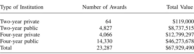
Table 1 shows the size of the HOPE Scholarship. The state awarded 23,287 schol-arships to the class of 2004, costing almost $68 million. Of those who qualified for and accepted the scholarship, 79 percent attended four-year colleges and the vast ma-jority of these attended public colleges.
B. Tennessee Postsecondary Education
Even before the TELS was enacted, 85 percent of Tennesseans going straight to col-lege attended one of the state’s nine four-year public universities, 13 two-year public colleges, 35 independent institutions, or 27 technology centers.2
The four-year public universities were competitive enough that a student on the margin of HOPE eligibility would have found peers of similar ability in the univer-sity system, but Tennessee’s ‘‘best and brightest’’ typically would not. Approximately 60 percent of 2004 Tennessee freshmen at Tennessee four-year public colleges re-ceived lottery scholarships. Academically, the four-year public colleges range from the historically black Tennessee State University, at which the middle 50 percent of students score between 16 and 21 on the ACT (equivalent to 760 to 1010 on the SAT) to the flagship, the University of Tennessee-Knoxville, at which the middle 50 percent of students score 20 to 27 on the ACT (equivalent to 940 to 1230 on the SAT). While the size of the individual HOPE awards was comparable to many other states’ scholarship programs, students planning to attend a public university could not have expected the HOPE Scholarship to cover their entire cost of attendance. In the year before the TELS was implemented, tuition and fees alone of the public four-year universities ranged from $500 to $1,500 more than the value of the HOPE Scholarship. For two-year colleges tuition and fees ranged from $550 to $600 more than the value of the scholarship.
C. Research on Merit Aid in Other States
Many papers analyze the effects of broad-based merit scholarship programs on stu-dent behavior. Dynarski (2004) analyzes programs in seven Southern states (not in-cluding Tennessee’s) using CPS data and finds large effects on college matriculation. In the aggregate, these programs increased the probability that students from these states would enroll in college by 4.7 percentage points, primarily by increasing the probability of enrolling at a public college.
Cornwell, Lee, and Mustard (2005 and 2006), Cornwell and Mustard (2006), and Cornwell, Mustard, and Sridhar (2006) find that the Georgia HOPE program in-creased students’ desire to attend Georgia colleges, particularly elite colleges. There was a significant increase in the number of students attending Georgia col-leges after the scholarship was implemented, specifically at four-year public and private Georgia colleges and HBCUs, while the acceptance rates of Georgia col-leges and the yield rates of elite Georgia colcol-leges decreased relative to control schools. They also find that to retain HOPE funding while in college, in-state Uni-versity of Georgia students enrolled in fewer credits overall, withdrew from more classes, took fewer math and science classes, and switched to easier majors than their out-of-state peers.
Less attention has been paid to these scholarships’ effects on high school achieve-ment. However, Henry and Rubenstein (2002) do indirectly show that the Georgia HOPE program increased Georgia high school achievement. They argue that the HOPE program increased high school grades among Georgia students entering Georgia public colleges, but SAT scores did not decrease relative to grades for this group, so the in-crease in grades must have been a result of improved achievement, not grade inflation.
III. Data Description
The data for this analysis come from a unique set of individual re-cords assembled from the administrative files of the ACT Corporation. The data in-clude a broad cross-section of observations on students who took the ACT and planned to graduate high school in 1996, 1998, 2000, and 2004: One out of every four Cauca-sians, one out of every two minorities, and every student who either listed their race as ‘‘multiracial’’ or ‘‘other’’ or failed to provide a race. I limit the sample to the 24 states3 in which the flagship university received more ACT than SAT scores, because the Table 1
College Choices of HOPE Scholarship Winners
Type of Institution Number of Awards Total Value
Two-year private 64 $119,000
Two-year public 4,827 $8,737,515
Four-year private 4,066 $12,799,297
Four-year public 14,330 $46,273,678
Total 23,287 $67,929,490
Notes: These figures only include students from the class of 2004. The data come from personal correspon-dence with Robert Anderson at the Tennessee Higher Education Commission.
students who take the ACT in states where the ACT is not the primary college entrance exam are not expected to be representative of the states’ potential college-goers. In the analysis of college preferences, I use only data from 1998, 2000, and 2004 since stu-dents graduating high school in 1996 could not send complimentary score reports to as many schools as in later years. Finally, in my analysis of score-sending, I omit the 13.6 percent of students who did not send their scores to any colleges.
Considering only these 24 states, there is still a large sample: 997, 346 records for the four years and over 225,000 in each year. The sample from Tennessee is large— there are 58,595 observations in total, with over 14,400 individuals in each year— and representative of the state’s college-goers—over 87 percent of the state’s high school seniors took the ACT in 2004.
I observe each student’s composite ACT score the last time she took the exam,4 stated preferences regarding aspects of her desired college, demographic, and other background information, and up to six colleges to which she sent her score.5Students indicate the colleges they’d like their scores sent to when they register for the test6 and indicate the state, number of years, institutional control, and maximum tuition of their desired college on test day. The background information is very detailed and includes gender, race, family income, classes taken, extracurricular activities, and out-of-class accomplishments.
The analysis in this paper differs from studies that analyze improvements in high school grades, which may confound changes in student achievement and incentives for grade inflation, because the ACT is an objective, nationally administered test. The extremely rich background information allows me to conclude that my results are not due to a changing pool of test-takers. However, I cannot conclude that the increases in ACT scores reflect human capital accumulation. Students could have increased their score as a result of developing ACT-specific human capital, getting more sleep the night before the exam, or exploiting the randomness in test questions by retaking the test until receiving their desired score. I cannot rule out the first two explanations, but I do use data on the traditional gains from retesting to show that the effect is too large to plausibly be generated by increased retesting alone.
Card and Krueger (2005) suggest that score-sending data is a good proxy for application data. They find that the number of SAT scores sent to a particular col-lege is very highly correlated with the number of applications it receives. Using score-sending data to measure college preferences has become common in the lit-erature.7 However, additionally analyzing students’ stated college preferences allows me to detect any changes in preferences over colleges within their appli-cation portfolios that would not be evident from examining score-sending or ap-plication data alone.
4. Despite my best efforts to procure data on how many times students took the ACT, their scores on pre-vious test sittings, and even aggregate information on retesting rates, I was only able to obtain a student’s score the last time she took the ACT.
5. Observing only six colleges to which students sent their scores does not practically limit my knowledge of student preferences as over 98% of students who sent test scores sent five or fewer.
6. After summer 1997, stundents could send four score reports for free, with each additional report costing $6 in 1998 and 2000 and $7 in 2004.
IV. Impact of the TELS on ACT Score
Tennessee students increased their ACT scores from below 19 to 19, 20, and 21 as a result of the TELS. This is evident in graphically comparing the dis-tribution of test scores in Tennessee from 2004 with disdis-tributions in earlier years and in difference-in-difference regressions. The results are incredibly robust.
A. Graphical Analysis
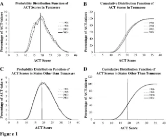
Figures 1a, 1b, 1c, and 1d show the probability and cumulative distributions of test scores in Tennessee and comparison states for each year. They show the 2004 distribution marks a clear departure from the other years in Tennessee, but not in the rest of the country.
The first analytic question is whether the change in the distribution of test scores cap-tures changes in the performance of test-takers or changes in the composition of the pool of test-takers. To control for differential selection into test-taking in the different years, I use a procedure developed by Dinardo, Fortin, and Lemieux (DFL), reweight-ing the 1996, 1998, and 2004 distributions so that they represent the counterfactual test-score distributions that would have prevailed if the same pool of students had taken the ACT in those years as in 2000.8I construct the counterfactual distribution for each year separately, pooling the observations from 2000 and that year, running a probit regres-sion of the year of the observation (2000¼1) on control variables and reweighting that year’s data by the ratio of the fitted value to the fitted value’s additive inverse. Appendix A has a mathematical explanation of the reweighting procedure.
I use many control variables in addition to state and year dummies, including in-formation on the students’ academic and extracurricular activities and dummies for whether each of the control variables is missing.9Because students’ academic and extracurricular records are potentially affected by the TELS, I reperform the analysis using only fully exogenous variables as controls. The results are very similar.
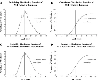
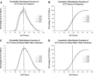
Figures 2a through 2d show how this reweighting procedure changes the test-score distributions for Tennessee and the rest of the country in 2004, while Figures 3a through 3d are replications of Figures 1a through 1d using the reweighted distributions. The graphs show that the change in the score distribution in 2004 was a result of actual score improvement and not solely a result of differential selection into test-taking. Figures 3a and 3b show that the only change in the Tennessee distribution from previous years was the change theory predicts— a shifting of mass from below 19 to 19 or just above. There is almost no change in the distribution of scores above 21.
8. This is very similar to the estimator proposed by Barsky et al. (2002) in their exploration of the black-white wealth gap.
To quantify the differences in the test-score distributions, I use Kullback and Leibler’s (1951) divergence function:
DKLðPkQÞ ¼+ i
PðiÞ3log PðiÞ
QðiÞ
!
;
ð1Þ
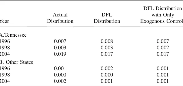
to calculate the divergence of the 2000 distribution (P) from the other years’ actual distributions, reweighted distributions, and distributions reweighted using only exog-enous controls (Q). The results are presented in Table 2. For states other than Ten-nessee, the divergences are small and fairly similar across years. For TenTen-nessee, the divergences of the 2004 population from the 2000 population are more than dou-ble the divergences between 2000 and any other year.
B. Regression Analysis
Using an indicator variable for whether the student scored 19 or higher on the ACT as the dependent variable (yist), I estimate difference-in-difference regressions
compar-ing the change in ACT scores in Tennessee in 2004 to the change in scores in other Figure 1
Actual Distributions of ACT Scores
states. I estimate the effect using both an OLS and probit specification, estimating Equations 2 and 3, respectively:
yist¼b0+b1TELSst+b2Xist+ds+dt+eist
ð2Þ
yist¼Fðb0+b1TELSst+b2Xist+ds+dtÞ+eist:
ð3Þ
HereTELSstis an indicator for whether the student lived in a state and year (Tennes-see in 2004) when the TELS was in effect andFrepresents the standard normal cu-mulative distribution function. The coefficient of interest in both cases is b1. The
termsdsanddtare state and year fixed effects respectively andeistis an idiosyncratic error term. I consider several different specifications forXist, the control variables. Standard errors are clustered at the state-year level.
Figure 2
Actual Distributions of ACT Scores Compared to Distributions Generated by Multivariate Reweighting
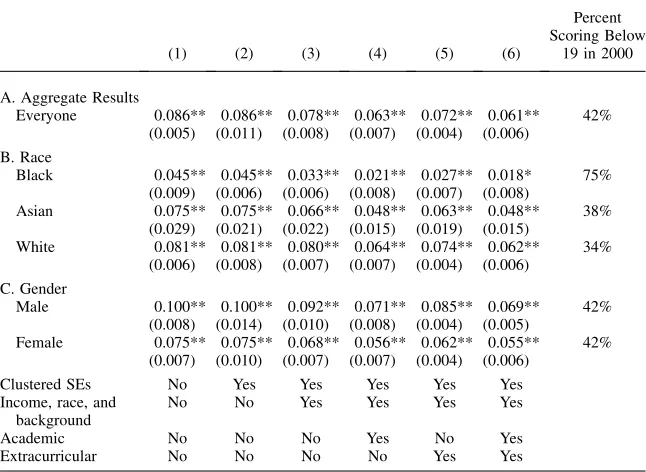
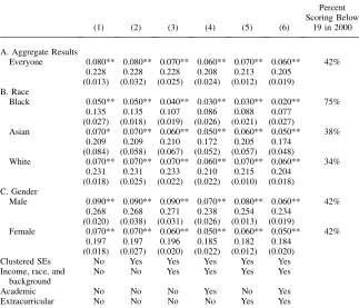
Results from estimating Equations 2 and 3 are presented in Tables 3 and 4, respec-tively. In Table 4, the first row in each cell contains the average of the marginal effects for each observation in the sample while the second and third rows in each cell are the estimated coefficient and standard error. The impact of the TELS is clear: Every coefficient in the tables is positive and significant at the 5 percent level and over 95 percent are significant at the 1 percent level. As more controls are added, the measured impact of the program decreases; however, it still remains large and significant. The coefficient also remains large and significant after the many robust-ness checks described in Appendix B. The results from these robustrobust-ness checks are displayed in Appendix Table A1.
For the whole population, the OLS coefficient is 0.061 when all controls are in-cluded and 0.079 when only the strictly exogenous controls are inin-cluded, signifying that 6.1 percent and 7.9 percent of Tennessee students increased their score to 19 or higher as a result of the TELS, respectively. These estimates are similar in magnitude to the actual 7.2 percent increase in the number of Tennessee students who scored 19 or higher before and after the TELS was implemented.
Figure 3
Distributions of ACT Scores Generated by Multivariate Reweighting
C. Assessing the Magnitude of the Effect
A 6.1 percentage point increase in the number of students scoring 19 or higher is a large increase in test scores.10Because only 42.1 percent of Tennessee test-takers scored below 19 in 2000, this implies that one out of every seven Tennessee students who could have increased their score to 19 or higher did so. This may even under-state the change in achievement as some students may have increased their scores but not all the way to 19 and some students who would have scored 19 or higher even without the TELS worked to increase their scores because of uncertainty over how they would perform.
Further analysis suggests that despite the decrease in mass at scores as low as 12 and 13 in Figure 3a, only students who would have scored 15–18 without the TELS increased their scores to 19 or higher. Some students who would have scored below 15 without the TELS did increase their scores, but fell short of 19.
Table 2
Kullback-Leibler Divergences Between ACT Distributions
Year
Actual Distribution
DFL Distribution
DFL Distribution with Only Exogenous Controls
A.Tennessee
1996 0.007 0.008 0.007
1998 0.003 0.003 0.002
2004 0.019 0.017 0.017
B. Other States
1996 0.001 0.002 0.001
1998 0.000 0.000 0.001
2004 0.002 0.001 0.001
Notes: Each cell in Panel A gives the Kullback-Leibler divergence between the actual Tennessee 2000 distribution of ACT scores and either the actual Tennessee distribution for the year indicated, the Tennessee distribution cre-ated using the DFL technique and all the control variables, or the Tennessee distribution crecre-ated using the DFL technique and only the fully exogenous controls. Panel B is the same for all states other than Tennessee. Exogenous controls are state and year fixed effects, income dummies, race dummies, and five background variables. The ad-ditional controls are eight aspects of the student’s academic history and four aspects of the student’s extracurricular participation. The specific controls are listed in Footnote 9. The data come from the ACT database.
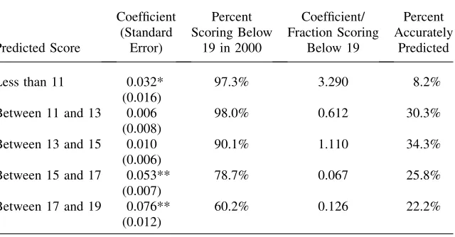
To determine whether students who would have earned low ACT scores increased their scores to 19 or higher, I first predict the ACT score students would have re-ceived without the TELS using data from 1996, 1998, and 2000 and all of the control variables. Then I estimate Equation 2 separately for students predicted to have dif-ferent ACT scores. Table 5 shows that the coefficients for students predicted to score below 15 are small and insignificant, but students predicted to score 15–17 and 17– 19 saw 5.3 and 7.6 percentage point increases in the probability of scoring 19 or higher respectively. Column 3, which attempts to account for the prediction error, suggests that 6.7 percent and 12.6 percent of students who would have scored in these ranges increased their scores above the threshold.
Though no information is available on changes in retesting rates, these effects are too large to be a function of students simply retaking the test. An ACT Research Table 3
The Effect of the TELS on Scoring 19 or Higher on the ACT: OLS Regressions
(1) (2) (3) (4) (5) (6)
Percent Scoring Below
19 in 2000
A. Aggregate Results
Everyone 0.086** 0.086** 0.078** 0.063** 0.072** 0.061** 42% (0.005) (0.011) (0.008) (0.007) (0.004) (0.006)
B. Race
Black 0.045** 0.045** 0.033** 0.021** 0.027** 0.018* 75% (0.009) (0.006) (0.006) (0.008) (0.007) (0.008)
Asian 0.075** 0.075** 0.066** 0.048** 0.063** 0.048** 38% (0.029) (0.021) (0.022) (0.015) (0.019) (0.015)
White 0.081** 0.081** 0.080** 0.064** 0.074** 0.062** 34% (0.006) (0.008) (0.007) (0.007) (0.004) (0.006)
C. Gender
Male 0.100** 0.100** 0.092** 0.071** 0.085** 0.069** 42% (0.008) (0.014) (0.010) (0.008) (0.004) (0.005)
Female 0.075** 0.075** 0.068** 0.056** 0.062** 0.055** 42% (0.007) (0.010) (0.007) (0.007) (0.004) (0.006)
Clustered SEs No Yes Yes Yes Yes Yes
Income, race, and background
No No Yes Yes Yes Yes
Academic No No No Yes No Yes
Extracurricular No No No No Yes Yes
Report using data from 1993 (Andrews and Ziomek 1998) found that 36 percent of students retook the ACT nationally. Eleven percent of those scoring 15 or 16 and 43 percent of those scoring 17 or 18 increased their score to 19 or higher on their second attempt. A back-of-the-envelope calculation shows that to get effects as large as seen here, there would need to be a 61 percentage point increase in retesting among stu-dents who scored 15–16 on their first attempt and a 29 percentage point increase in retesting among those who scored 17–18. Assuming the fraction of students retaking the ACT was constant across ACT scores, 97 percent of students scoring 15 and 16 Table 4
The Effect of the TELS on Scoring 19 or Higher on the ACT: Probit Regressions
(1) (2) (3) (4) (5) (6)
Percent Scoring Below
19 in 2000
A. Aggregate Results
Everyone 0.080** 0.080** 0.070** 0.060** 0.070** 0.060** 42% 0.228 0.228 0.228 0.208 0.213 0.205
(0.013) (0.032) (0.025) (0.024) (0.012) (0.019) B. Race
Black 0.050** 0.050** 0.040** 0.030** 0.030** 0.020** 75% 0.135 0.135 0.107 0.086 0.088 0.077
(0.027) (0.018) (0.019) (0.026) (0.021) (0.027)
Asian 0.070* 0.070** 0.060** 0.050** 0.060** 0.050** 38% 0.209 0.209 0.210 0.172 0.205 0.174
(0.084) (0.058) (0.067) (0.052) (0.057) (0.048)
White 0.070** 0.070** 0.070** 0.060** 0.070** 0.060** 34% 0.231 0.231 0.233 0.210 0.215 0.204
(0.018) (0.025) (0.022) (0.022) (0.010) (0.018) C. Gender
Male 0.090** 0.090** 0.090** 0.070** 0.080** 0.060** 42% 0.268 0.268 0.271 0.238 0.254 0.234
(0.020) (0.038) (0.031) (0.026) (0.013) (0.019)
Female 0.070** 0.070** 0.060** 0.050** 0.060** 0.050** 42% 0.197 0.197 0.196 0.185 0.182 0.184
(0.018) (0.027) (0.020) (0.022) (0.012) (0.020)
Clustered SEs No Yes Yes Yes Yes Yes
Income, race, and background
No No Yes Yes Yes Yes
Academic No No No Yes No Yes
Extracurricular No No No No Yes Yes
would have had to retake the ACT to see effects this large. This is too large to be plausible.11Since students often study between test dates, even if this effect could be explained only by retesting, the gains still would have probably partially been a result of increased human capital.
D. Impact of the TELS on Different Subgroups
Tables 3 and 4 also display the results from restricting the estimation of Equations 2 and 3 to different subgroups. They show that African-Americans were significantly less responsive to the TELS than Asians and Caucasians, and males were slightly more responsive than females.
The results in Table 3 suggest an African-American who would have scored below 19 without the TELS was over five times less likely than an Asian and seven times less likely than a Caucasian to increase her score to 19 or higher: The point estimate for blacks is smaller than for other groups and the fraction scoring below 19 is larger. Table 5
Effect of TELS on Students with Different Predicted Academic Ability
Predicted Score
Less than 11 0.032* 97.3% 3.290 8.2%
(0.016)
Between 11 and 13 0.006 98.0% 0.612 30.3%
(0.008)
Between 13 and 15 0.010 90.1% 1.110 34.3%
(0.006)
Between 15 and 17 0.053** 78.7% 0.067 25.8%
(0.007)
Between 17 and 19 0.076** 60.2% 0.126 22.2%
(0.012)
Notes: ACT scores are predicted by an OLS regression using observations from 1996, 1998, and 2000, all the controls listed in Footnote 9, and state and year dummies. The results in the four data columns are lim-ited to students predicted to score in the range indicated in the leftmost column. The first data column gives the coefficient and standard error (clustered at the state-year level) from an OLS regression. The dependent variable is an indicator for whether the student scored 19 or higher on the ACT; all controls listed in Foot-note 9 plus state and year dummies are included. The far right-hand column indicates the percentage of students predicted to be in that range in 1996, 1998, and 2000 who did score in the range (for example, for students predicted to be in the 11–13 range, the percentage of students scoring 11 or 12). One asterisk indicates the result is significant at the 5 percent level and two asterisks indicate the result is significant at the 1 percent level. Data come from the ACT database.
Part, but not all, of this disparity in apparent responsiveness is due to the fact that African-Americans scoring below 19 scored, on average, lower than the other racial groups, so they would have had to increase their score by more to reach the cutoff of 19. However, a higher percentage of Tennessee blacks score between 15 and 18 than Tennessee whites, so if blacks and whites were equally affected by the TELS, the point estimate for blacks should be higher than the point estimate for whites. Repeating the analysis in Table 5 separately for blacks and whites suggests African-Americans were at least three times less responsive to the TELS than Caucasians.
Males were slightly more responsive to this program than females. The coeffi-cients of different specifications of Equation 2 are 25 percent to 37 percent higher for males than females. In pooled data the interaction term between being male and the presence of the TELS is positive and significant in every specification while the score distributions of males and females before the TELS were very similar. This result is interesting in light of several papers that find larger effects of financial incen-tives on educational attainment and performance for females (for example, Angrist, Lang, and Oreopoulos 2006; Angrist and Lavy 2002; and Dynarski 2005).
V. Impact of the TELS on College Applications
The TELS did not affect where students sent their ACT scores or stu-dents’ stated college preferences. I analyze stustu-dents’ preferences for in-state versus out-of-state, four-year versus two-year, and four-year state versus two-year in-state colleges as well as the tuition students were willing to pay and find no robust effect of the TELS.
For each type of school listed above, I estimate Equation 2 separately using the total number of scores the student sent to that type of college, a dummy variable for whether the student sent any score to that type of college, and the student’s pref-erence for that type of college as dependent variables. I also use the maximum tuition the student reports being willing to pay and the average tuition of colleges she sent scores to as dependent variables.12Tables 6 and 7 present the results for the whole sample, students who scored 19 or higher on the ACT, students who scored below 19, and students who scored below 19 and reported a GPA below 3.0. I include all of the control variables and cluster standard errors at the state-year level.
While these subgroups are endogenous, if the results are due to the TELS, we would expect students scoring 19 or higher to be much more responsive than students who are likely ineligible. The results are not driven by the endogeneity of the subgroups; they
Two-Year vs. Four-Year Colleges
Full Sample
ACT at Least 19
ACT Below 19
ACT Below 19 and GPA Less Than 3.0
Mean in 2000 Tennessee
A. Robustness Check
Total scores sent 20.043 20.081 20.002 0.017 2.99
(0.047) (0.053) (0.032) (0.035)
B. In-State vs. Out-of-State Colleges
Total in-state colleges 20.084 20.097 20.031 0.005 2.08
(0.052) (0.057) (0.039) (0.042)
Any in-state college 20.005* 20.004 0.000 0.002 0.79
(0.002) (0.003) (0.002) (0.002)
Total out-of-state colleges 0.041** 0.015 0.029* 0.012 0.91
(0.014) (0.015) (0.014) (0.016)
Any out-of-state college 0.023** 0.013 0.018* 0.011 0.45
(0.008) (0.008) (0.009) (0.008)
Prefer to attend college in-state 20.012 20.021* 0.001 0.011 0.72
(0.007) (0.010) (0.006) (0.006)
C. Four-Year vs. Two-Year Colleges
Total four-year colleges 0.029 20.033 0.064** 0.098** 2.58
(0.034) (0.043) (0.021) (0.023)
Any four-year college 0.002* 0.000 20.001 20.003 0.83
(0.001) (0.000) (0.002) (0.003)
Total two-year colleges 20.073** 20.048** 20.066** 20.081** 0.41
(0.016) (0.012) (0.019) (0.023)
Pallais
Any two-year college 20.039** 20.030** 20.020 20.017 0.32
(0.011) (0.009) (0.012) (0.015)
Prefer to attend four-year college 0.033** 0.013** 0.029** 0.041** 0.84
(0.007) (0.004) (0.011) (0.014)
Notes: Each cell in the first four columns of data gives the coefficient and standard error of a separate regression on the dependent variable listed in the left-hand column. Each regression is limited to the individuals indicated by the column heading. The first four specifications in Panels B and C relate to scores sent whereas the last relates to stated preferences. All of the controls listed in Footnote 9 as well as state and year dummies are included and standard errors are clustered at the state-year level. One asterisk indicates the result is significant at the 5 percent level and two asterisks indicate the result is significant at the 1 percent level. The right-most column gives the mean of each variable for the sample of 2000 Tennessee test-takers. Data on score-sending, preferences, GPA, and ACT score come from the ACT database and data on the level and location of the colleges comes from the IPEDS.
The
Journal
of
Human
Tuition Preferences
Full Sample
ACT at Least 19
ACT Below 19
ACT Below 19 and GPA Less Than 3.0
Mean in 2000 Tennessee
A. Four-Year In-State vs. Two-Year In-State Colleges
Total four-year in-state colleges 20.016 20.053 0.033 0.084** 1.72
(0.038) (0.048) (0.024) (0.024)
Any four-year in-state college 20.003 20.006* 0.000 0.003 0.76
(0.002) (0.003) (0.002) (0.003)
Total two-year in-state colleges 20.068** 20.043** 20.064** 20.080** 0.36
(0.015) (0.010) (0.019) (0.023)
Any two-year in-state college 20.037** 20.029** 20.018 20.014 0.29
(0.011) (0.008) (0.013) (0.015)
Prefer four-year in-state college 0.012** 20.009 0.015** 0.033** 0.58
(0.003) (0.007) (0.005) (0.008)
B. Tuition
Preferred maximum tuition 251.8** 109.1 129.7* 53.5 $4,016.97
(31.6) (61.0) (56.6) (54.5)
Average tuition of colleges scores sent to 235.8** 76.0 227.3** 266.0** $9,141.88
(62.9) (42.7) (46.1) (52.2)
Notes: Each cell in the first four columns of data gives the coefficient and standard error of a separate regression on the dependent variable listed in the left-hand column. Each regression is limited to the individuals indicated by the column heading. The first four specifications in Panel A relate to scores sent whereas the last relates to stated preferences. All of the controls listed in Footnote 9 as well as state and year dummies are included and standard errors are clustered at the state-year level. One asterisk indicates the result is significant at the 5 percent level and two asterisks indicate the result is significant at the 1 percent level. The right-most column gives the mean of each variable for the sample of 2000 Tennessee test-takers. Data on score-sending, preferences, GPA, and ACT score come from the ACT database and data on the level, location, and tuition of the colleges comes from IPEDS. Tuition is the in-state tuition in 2004-05 if the student lived in the same state as the college and the out-of-state tuition in 2004-05 if the student lived in a different state.
Pallais
are the same when ACT score and GPA are predicted using data before the TELS and the subgroups restricted based on those variables.
Panel A of Table 6 shows that the number of scores sent did not change signifi-cantly either in the aggregate or for any of the subgroups examined, allowing us to more easily interpret changes (or the lack thereof) in score-sending as changes (or lack thereof) in preferences. Panel B shows that the TELS did not induce students to prefer in-state colleges more strongly. In fact, while not all significant, the point estimates all indicate students were less likely to prefer in-state as compared to out-of-state colleges: Students sent fewer scores to in-state colleges, more scores to out-of-state colleges, and were less likely to say they wanted to attend college in-state. This is not due to preferences of students who were ineligible for the schol-arship: The point estimates for students scoring 19 or higher are all signed in the ‘‘wrong’’ direction as well.
While results from the entire sample indicate that Tennessee students increased their preference for four-year as opposed to two-year schools, the point estimates for students scoring 19 or higher, while not significant, indicate these students sent fewer scores to four-year colleges. It was only students scoring below 19 (including those with GPAs below 3.0) who sent scores to more four-year colleges in 2004. Moreover, while students scoring 19 or higher did realize decreases in both the total number of two-year colleges they sent scores to and their preferences for four-year colleges, these changes were only about half and one-third as large, respectively, as those realized by students with ACT scores below 19 and GPAs below 3.0.
While preferences for four-year colleges could theoretically decrease if students began to prefer two-year in-state colleges over four-year out-of-state colleges (an admittedly very unusual response), the predictions indicate unambiguously that the TELS should increase the preference for four-year in-state colleges. However, the point estimates for students scoring 19 or higher indicate that these students were less likely to send scores or express preferences for attending four-year in-state colleges.
Finally, there was no effect of the TELS on the tuition students were willing to pay. In the aggregate, Tennessee students both said they were willing to pay higher tuition and sent their scores to more expensive schools in 2004. However, students scoring 19 or higher were the only group not to see a significant increase in the actual tuition of colleges scores were sent to and the point estimate for this group is approx-imately one third of those for the other two groups. They also did not report larger increases in the tuition they were willing to pay than the other groups.
While students could have changed their college preferences later in the applica-tion process, this analysis provides strong evidence that students had not changed their college preferences as a result of the TELS by the time they took the ACT. This section shows the value of using micro data with detailed background characteristics to analyze the difference in score-sending.
VI. Conclusion
to win the scholarship based on their grades and were interested in attending a Tennessee college. It also decreased the cost of attending in-state as compared to out-of-state and four-year in-state as compared to two-year in-state colleges for scholarship winners.
The TELS did not induce scholarship winners to change their college preferences. Students did respond to the scholarship, however. Graphically, it is clear that students’ scores increased sharply around the threshold of 19 while difference-in-difference regressions show that the probability a given student would score 19 or higher on the ACT increased by 6 percent to 8 percent in the first year of the program. This effect is extremely robust. It is also a very large increase, implying that one out of every seven students who could have increased their scores to 19 or higher did so as a result of the TELS. African-Americans responded very little to the scholarship incentive while males were more responsive than females.
The large increase in ACT scores induced by the TELS show that policies that reward students for their academic performance can potentially generate large improvements in high school achievement. The fact that this performance improve-ment is too large to result from students simply retaking the test suggests that it may likely indicate true human capital accumulation. However, it remains to be seen whether this is ACT-specific human capital, such as learning the directions for the test, or whether this is human capital that will positively affect other outcomes.
APPENDIX 1
Mathematical Explanation of the Multivariate Reweighting Procedure
Letf(ACTjz,t,TELS) be the distribution of ACT scores for students with a set of ob-servable characteristicsz, in yeart, in a state of the world where the TELS is in place (TELS ¼1) or a state of the world where it is not (TELS¼0). LetdF(zjt) be the distribution of attributes z in the pool of ACT-takers in year t. Then, the actual dis-tribution of scores in 2004 is
Z
fðACTjz;t¼2004;TELS¼1Þ3dFðzjt¼2004Þ
ð4Þ
while the distribution of scores that would have prevailed in 2004 if the population of test-takers was the same in 2004 as it was in 2000, is
Z
fðACTjz;t¼2004;TELS¼1Þ3dFðzjt¼2000Þ
ð5Þ
I define the reweighting function
uzðzÞ ¼dFðzjt¼2000Þ
dFðzjt¼2004Þ ð6Þ
Z
fðACTjz;t¼2004;TELS¼1Þ3dFðzjt¼2000Þ ¼ Z
fðACTjz;t¼2004;TELS¼1Þ3dFðzjt¼2004Þ3uzðzÞ:
ð7Þ
which is practically estimated by reweighting each observation in the 2004 pool by the relevant value of uˆzðzÞ, estimated as described in the text.
Appendix 2
Robustness Checks for the Effect of the TELS on ACT Scores
The difference-in-difference results are extremely robust in terms of both the magni-tude and significance of the effect. Tables 3 and 4 show that the results are not sen-sitive to the specific controls or specification chosen. In Table A1, I show they are not due to serial correlation of ACT scores within states over time or the fact that I only analyze the behavior resulting from one state’s policy change.
Serial correlation is not as likely to be a problem in my analysis as many other differences-in-differences papers because I use a short time series with only four periods (see Bertrand et al. 2004). Moreover, regressing the mean residuals within a state for a given year on their lagged value produces negative coefficients, suggest-ing that in fact the reported standard errors may be too high.
The coefficient is of similar magnitude and still significant when state-specific lin-ear time trends are added and standard errors are clustered at the state level. It remains large and significant when the data are collapsed down to the state-year level and even, in all but one specification, when data are collapsed to the state-year level when state-specific linear time trends are added.13Even collapsing the data into two
observations by state, one before and one after the TELS was implemented, yields a highly significant estimate which indicates a 7.6 percentage point increase in Tennes-see students scoring 19 or higher as a result of the TELS.
Conley and Taber (2006) show that if the number of states whose policy changes stays fixed even when the number of states used as controls and the number of stu-dents in a state approaches infinity, the program effect estimated by a difference-in-difference regression is not consistent. However, the last two sets of rows in Table A1 show that this is not driving my results. I use the consistent estimator of p-values that they suggest on both the individual and state-year data and the p-values are all below 0.05.14The procedure for constructing this estimator is as follows.
Conley and Taber start with the following model of data at the state-year level:
13. The only coefficient that isn’t significant is a coefficient in a regression that estimates 89 coefficients with 96 observations.
(1) (2) (3) (4) (5) (6)
A. Residual Regressions
Basic specification 20.270 20.270 20.254** 20.298 20.269 20.295 (0.344) (0.344) (0.000) (0.193) (0.173) (0.173) Including state time trends 20.403** 20.403** 20.427** 20.496** 20.443** 20.502**
(0.075) (0.075) (0.082) (0.081) (0.088) (0.083) B. Individual-Level Regressions
Including state time trends 0.085** 0.085** 0.075** 0.074** 0.070** 0.074** (0.011) (0.014) (0.011) (0.013) (0.010) (0.013) Clustering at state level 0.092** 0.092** 0.078** 0.063** 0.072** 0.061**
(0.021) (0.021) (0.011) (0.008) (0.005) (0.005) C. State-Year Regressions
Basic specification 0.076** 0.076** 0.049** 0.042** 0.054** 0.048* (0.006) (0.006) (0.008) (0.015) (0.008) (0.019) Including state time trends 0.078** 0.078** 0.075** 0.059 0.053*
(0.013) (0.013) (0.018) (0.035) (0.025) D. State Pre/Postperiod Regressions
Basic specification 0.076** (0.005) E. Conley-TaberP-values
Individual-level regressions 0.043 0.043 0.043 0.000 0.000 0.000 State-year regressions 0.043 0.000 0.000 0.000 0.000 0.000
Clustered SE’s No Yes Yes Yes Yes Yes
Income, race, and background No No Yes Yes Yes Yes
Academic No No No Yes No Yes
Extracurricular No No No No Yes Yes
Notes: Each cell in the first four panels gives the coefficient and standard error of a separate regression, the specification of which is indicated by the leftmost column. In panels B, C, and D the dependent variable is an indicator for whether the student scored 19 or higher on the ACT. In Panel C the data is collapsed to the state-year level whereas in Panel D the data is collapsed to a pre-TELS and post-TELS observation for each state. Cells in Panel C and D are left empty when the model is not identified. In, Panel A, the dependent variable is the average state residual from estimating Equation 2 using the controls indicated by the column and the independent variables are the average residual from the previous year and a constant. Panel E computes Conley-Taber. (2006) p-values which correct for the fact that I only analyze one policy change. Their construction is explained in Appendix B. The bottom rows indicate the control variables included in the regression and whether standard errors are clus-tered. When standard errors are clustered, it is at the state-year level and when they are not, they are White’s robust standard errors. The specific control variables cor-responding to each category are listed in Footnote 9. One asterisk indicates the result is significant at the 5 percent level and two asterisks indicate the result is significant at the 1 percent level. Data come from the ACT database.
Pallais
Y˜jt¼ad˜jt+X˜#jtb+ ˜hjt:
ð8Þ
Here j indexes the state, t indexes the time period and tildes denote variables which are projections onto group and time indicators. For any variable Z, Z˜jt¼ Zjt2Zj2Zt2Z, whereZj,Zt, andZare the state, year, and overall mean of Z respec-tively. The variablesXjtare control variables that vary at the state-year level anddjtis the indicator for whether the policy was in effect at the time;hjtis the idiosyncratic error.
When the number of states who do change their policy (N0) is finite, but the
num-ber of states who do not (N1) grows large, the differences-in-differences estimator ˆa
converges in probability toa+ W, where
W¼+
The states that change their policies are indexed byjequal to 1 toN0; states which do
not realize a policy change are indexed byjequal toN0+ 1 toN1.
Assuming that the state-year errors are independent of any regressors and identi-cally distributed across state-year cells, a consistent analog estimator of the condi-tional cumulative distribution function ofWgiven the entire set ofd’s is
ˆ
where 1(.) is an indicator function.
I use this estimated cumulative distribution function and report Prðaˆ+W,0Þ ¼ PrðW,2aÞ ¼ˆ Gð2aÞˆ as thep-value directly for the regressions done at the state-year level as Conley and Taber suggest. For the individual level regressions, pre-sented in the line above, I also follow the suggestion of Conley and Taber. The regression model
Yi¼adjt+X#jtb+uj+gt+Z#id+mi;
ð11Þ
whereZiare controls that vary at the individual level andmiare idiosyncratic errors, can be estimated as
Yi¼ljðiÞt+Z#id+ei
ð12Þ
ljt¼adjt+X#jtb+uj+gt+hjt
ð13Þ
where ljt are the individual state-year fixed effects and hjt are errors. I estimate Equation 12, use the estimates for ljt as the dependent variables in Equation 13 and then calculate thep-value for each specification as in Equation 10.
affect this outcome much). While the TELS may cause students who do not send their scores to any in-state colleges to increase their ACT score as a result of spill-overs or uncertainty over whether they will want to attend an in-state college in the future, students who prefer to attend college in-state should have a larger response. This is the case. The coefficient from estimating Equation 2 is 60 percent larger for students sending scores to in-state colleges. Adjusting for the distribution of test scores before the TELS shows even stronger results: The coefficients from the regres-sions restricted to students in predicted ACT ranges are four times larger for students sending scores in-state. For these students, the Kullback-Leibler divergences for 2004 are ten times larger than those for any other year, while for students who did not send any scores in-state, the divergences for 2004 are only 1.4 times larger than those in other years.
References
Abraham, Katharine, and Melissa Clark. 2006. ‘‘Financial Aid and Students’ College Decisions: Evidence from the District of Columbia Tuition Assistance Grant Program.’’ Journal of Human Resources 41(3):578–610.
ACT Assessment Data: 1991–2004. ACT Corporation. Electronic Data.
Andrews, Kevin, and Robert Ziomek. 1998. ‘‘Score Gains on Retesting with the ACT Assessment.’’ACT Research Report Series98(7):1–36.
Angrist, Joshua, Daniel Lang, and Philip Oreopoulos. 2006. ‘‘Lead Them to Water and Pay Them to Drink: An Experiment with Service and Incentives for College Achievement.’’ NBER Working Paper 12790.
Angrist, Joshua, and Victor Lavy. 2002. ‘‘The Effect of High School Matriculation Awards: Evidence from Randomized Trials.’’ NBER Working Paper 9389.
Barsky, Robert, John Bound, Kerwin Charles, and Joseph Lupton. 2002. ‘‘Accounting for the Black-White Wealth Gap: A Nonparametric Approach.’’Journal of the American Statistical Association97(459):663–73.
Card, David, and Alan Krueger. 2005. ‘‘Would the Elimination of Affirmative Action Affect Highly Qualified Minority Applicants? Evidence from California and Texas.’’Industrial and Labor Relations Review58(3):416–34.
Cornwell, Christopher, Kyung Lee, and David Mustard. 2005. ‘‘Student Responses to Merit Scholarship Retention Rules.’’Journal of Human Resources40(4):895–917.
__________. 2006. ‘‘The Effects of State-Sponsored Merit Scholarships on Course Selection and Major Choice in College.’’ IZA Discussion Paper 1953.
Cornwell, Christopher, and David Mustard. 2006. ‘‘Merit Aid and Sorting: The Effects of HOPE-Style Scholarships on College Ability Stratification.’’ IZA Discussion Paper 1956. Cornwell, Christopher, David Mustard, and Deepa Sridhar. 2006. ‘‘The Enrollment Effects of
Merit-Based Financial Aid: Evidence from Georgia’s HOPE Scholarship.’’Journal of Labor Economics24(4):761–86.
Dinardo, John, Nicole Fortin, and Thomas Lemieux. 1996. ‘‘Labor Market Institutions and the Distribution of Wages, 1973–1992: A Semiparametric Approach.’’Econometrica 64(5):1001–44.
__________. 2005. ‘‘Building the Stock of College-Educated Labor.’’ NBER Working Paper 11604.
Henry, Gary, and Ross Rubenstein. 2002. ‘‘Paying for Grades: Impact of Merit-Based Financial Aid on Educational Quality.’’Journal of Policy Analysis and Management 21(1):93–109.
Integrated Postsecondary Education Data System: Data set Cutting Tool.
Kullback, Solomon, and Richard Leibler. 1951. ‘‘On Information and Sufficiency.’’Annals of Mathematical Statistics22(1):76–86.
Long, Mark. 2004. ‘‘College Applications and the Effect of Affirmative Action.’’Journal of Econometrics121(1-2):319–42.
Ness, Erik, and Brian Noland. 2004. ‘‘Targeted Merit Aid: Tennessee Education Lottery Scholarships.’’ Presented at the 2004 Annual Forum of the Association for Institutional Research, Boston: June 1.
Pallais, Amanda, and Sarah Turner. 2006. ‘‘Opportunities for Low Income Students at Top Colleges and Universities: Policy Initiatives and the Distribution of Students.’’National Tax Journal59(2):357–86.
Pope, Devin, and Jaren Pope. 2006. ‘‘Understanding College Choice Decisions: How Sports Success Garners Attention and Provides Information.’’ Virginia Polytechnic Institute. Unpublished.
Standard Research Compilation: Undergraduate Institutions. 2002. College Entrance Examination Board. Electronic data.
Statistical Abstract of Tennessee Higher Education 2003–2004.Tennessee Higher Education Commission.