www.elsevier.nl / locate / econbase
Supply side hysteresis: the case of the Canadian
unemployment insurance system
a ,* b
Thomas Lemieux , W. Bentley MacLeod a
Department of Economics, University of British Columbia, Vancouver, BC, V6T 1Z1, Canada H3C 3J7
b
Department of Economics /The Law School, University of Southern California, Los Angeles, CA90089-0253, USA
Abstract
This paper presents results from a 1971 natural experiment carried out by the Canadian government on the unemployment insurance system. At that time, the generosity of the UI system was increased dramatically. We find some evidence that the propensity to collect UI increases with a first-time exposure to the new UI system. Hence, as more individuals experience unemployment, their lifetime use of the system increases. This supply side hysteresis effect may explain why unemployment has steadily increased over the 1972–
1992 period, even though the generosity of unemployment insurance did not. 2000
Elsevier Science S.A. All rights reserved.
Keywords: Unemployment insurance; Learning; Incentives; Unemployment; Hysteresis
JEL classification: H53; J64; J65
1. Introduction
A recurrent theme in policy debates regarding social welfare programs is the relationship between benefits and the disincentives to work (Moffitt, 1982). In the case of unemployment insurance, there is a great deal of evidence suggesting that it tends to increase both the duration of unemployment and the probability of
*Corresponding author.
1
becoming unemployed. Moreover, work by Katz and Meyer (1990), Corak (1993) and Meyer and Rosenbaum (1996) find evidence that workers adjust their labor supply so that unemployment insurance may subsidize part-year work. Despite this micro-econometric evidence, there does not seem to be a direct relationship between unemployment insurance benefits and the recent secular rise in
unemploy-2
ment in the OECD . Lindbeck (1995) has pointed to social norms and the sluggish response of individual labor supply to changes in incentives as a potential source of ‘supply side hysteresis’ that may help explain this secular trend.
The goal of this paper is to build upon this idea, and see whether recent trends in the use of UI in Canada can be explained using a simple adaptive learning model. In a standard labor supply framework one supposes that changes in worker alternatives result in an immediate behavioral response. Moreover, whether or not the individual has had experience with the alternatives is irrelevant to his or her choice. However, there is a large body of evidence demonstrating that experience does matter for human decision making (e.g. Wickens, 1992).
It is well recognized in the economics literature that it takes time for individuals to find an optimal response, and hence short-run supply elasticities are likely to be
3
smaller than long-run elasticities. The issue that we wish to address in the study is the importance of this lagged adjustment in the case of labor supply responses to changes in the unemployment insurance (UI) parameters. A number of studies have shown that individuals adjust their labor supply as a function of the parameters of the system in the predicted direction. However, in the case of the Canadian UI system, UI use and unemployment increased steadily from 1971 until the 1990s, though during this period benefit level were constant or falling (see Figs. 1 and 2).
The hypothesis we wish to explore is that workers did not immediately respond to the large increase in benefits that occurred in 1971. Rather, when workers experienced unemployment for the first time, due to natural turnover or a recession, this exposed them to UI and caused them to begin exploring ways to use the UI system as a subsidy to part-year work. This was possible due to a number of rule changes that occurred in 1971. First, coverage of the UI system was expanded from 68 to 96% of the work force. The number of weeks of work needed to qualify for benefits was reduced from 30 weeks in a 2-year period to 8 weeks in a single year. The maximum number of weeks during which benefits could be received by a worker having worked the minimum number of weeks required to
1
See, for example, Topel (1983), Meyer (1990) for the United States, and Ham and Rea (1987) and Green and Riddell (1993) for Canada.
2
See, for example, Layard et al. (1991). 3
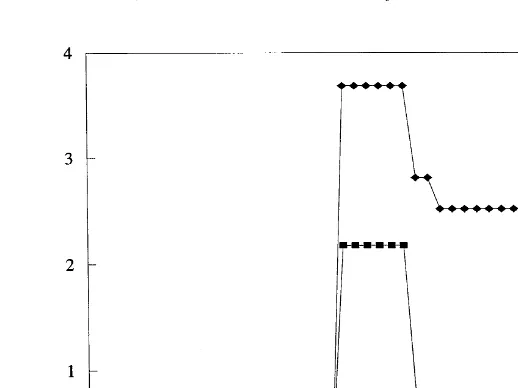
Fig. 1. UI subsidy rate for minimally qualified claimants.
qualify was increased from 15 to up to 44 weeks, depending on the regional unemployment rate (in high-unemployment regions benefits are more generous). The replacement rate was increased from 57% of previous earnings to 66% (or 75% if claimant had dependents). The generosity of the program is summarized by the subsidy rate (replacement rate3number of weeks of benefits for someone who has worked the minimum number of weeks to qualify / number of weeks needed to qualify) which is illustrated in Fig. 1 for the period 1951–1996.
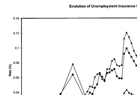
Fig. 2. Evolution of unemployment insurance use.
about 3% in 1972 to 5% in 1991, a 66% increase. This occurred even though the
4
incentives for use were either constant or decreasing.
To see how conditioning may help explain this observation, consider a cohort of workers that were working full year in 1971, the date of the large-scale change to UI. Over time more and more workers from this cohort will have experienced unemployment and possibly received some UI. We find that the probability that an individual will receive UI increases when he or she has had experience with the system in the past, implying that the fraction of workers receiving UI should also
5
increase over time, even though the parameters of the system are unchanged. This also creates a hysteresis effect during recessions. A recession increases the number of workers who leave full-year employment and experience unemployment and UI. The conditioning or learning effect that we identify implies that at the end of the recession, the equilibrium number of workers who are unemployed should be greater, and hence the economy should not return to its pre-recession equilibrium level of employment. This may account for the rising trend in the unemployment rate illustrated in Fig. 2.
4
The earnings replacement rate of UI was reduced to 60% in 1978 (from 66% in 1971), 57% in 1990, and 55% in 1993; the minimum qualifying period was extended to 10 weeks in 1978 (from 8 weeks in 1971), and to 12 weeks in 1990.
5
To ensure that we are identifying a behavioral change rather than a structural change in the economy, we follow the behavior of individual workers using a large administrative data set. In addition to the usual controls, we are able to control for individual effects, year effects and industry effects. Using a random effects probit model, we find some evidence that first-time treatment with the UI system permanently increases future use. In Section 2 we present a discussion of the model. Section 3 presents the administrative data set used in this study, while Section 4 provides some simple results using a difference-in-differences approach. Section 5 discusses the main estimation strategy. The results are discussed and summarized in Sections 6 and 7.
2. The effect of UI generosity on UI recipiency
For purposes of exposition it is useful to present a simple model that captures many of the incentive effects of UI. Suppose that at time t all workers are completely characterized by their base productivity denotedut, and their value of home production denoted by u . The base productivity of a person is a compositet
variable representing the market value of education, occupation choice and innate skills. Since this variable represents a market value, it will vary over time due to on-the-job training, technical change, etc.
In addition to a worker’s base productivity, the wage of a worker is also affected by business cycle shocks, including seasonal shocks. Lettinght denote the size of this shock in period t, suppose that the wage of a worker is given by:
wt5u 1ht t (1)
Abstracting away from the time required for search, individuals choose employ-ment if and only if the wage is greater than the value of home production or
wt$u . Let Et s dh 5 u
h
s ,uduu 1h $u denote the set of worker characteristics thatj
would result in full-time employment in the absence of UI, while Os dh denotes the set of characteristics of workers who are out of the labor force.
Now consider what happens when UI is introduced in the model. Suppose that once an individual has x weeks of insured employment, she or he is eligible for y weeks of benefits equal to a fractiona of the previous wage. An individual with characteristics (u,u) considers one of the following three options (with the t subscripts dropped for convenience):
1. Work full year at a wage of w5u 1h. 2. Exit the labor force to receive a benefit of u.
6
benefits until exhaustion before beginning to work again. Lettingd 5x /(x1y)
be the fraction of time the worker must be employed to earn y weeks of benefits, the return to the individual is given by ui5dw1(12d)(u1aw)5
(d 1(12d)a)w1(12d)u. Let us call a worker that follows this strategy a part-year worker.
Individuals choosing to work part-year are from the set of characteristics:
Ush,d,a 5 ud
h
s ,uduui$max w,uh jj
(2)Notice that the addition of a UI system creates an incentive for some full-time employees to work part-year, and for some individuals who are out of the labor market to work part-year. The implications of parameter changes are summarized in the following proposition.
Proposition 1. Decreasing the entry requirement,d, or increasing the replacement
rate,a, has the following effects: (i ) Participation in the labor force increases. (ii )
The number of individuals receiving UI per year increases.
9
Proof. This result follows immediately from the observation that ford # d and
9 9 9 9 9
a $ a then Ush,d, ad7U
s
h,d ,ad
, with strict membership ifsd, ad±s
d ,ad
.h
If workers receiving UI report that they are looking for work, then an increase in UI generosity (lowerd or highera) increases both measured unemployment and labor force participation. This observation is consistent with the finding of Card and Riddell (1993) that though unemployment grew in Canada during the 1980s, so did labor force participation, particularly by women. An actual example is employment in the arts. In Canada there a great deal of sectorial employment, such as summer theater companies, that permits the entry of businesses that survive because its employees are able to receive UI during the winter months. It is worth emphasizing that the supply side behavior described here must also be consistent with changes in demand side behavior. Firms, particularly those employing seasonal workers, are also learning and would increase their demand for seasonal workers in response to their increased supply. However, our panel does not have data on firms, and therefore we cannot identify the impact of UI changes on labor demand.
6
2.1. Hysteresis
When the major change to the UI system occurred in 1971, this increased the incentives for individuals to subsidize part-year employment with UI. Fig. 2 shows that the rate of use of UI increased sharply between 1971 and 1972. It then followed an upward trend between 1972 and 1992 even though the underlying incentives (subsidy rate) were constant or declining. The main goal of this paper is to investigate whether individuals permanently change their behavior after a bout of experience receiving UI.
While the immediate impact of the change in rules is consistent with the standard economic model of incentives, the fact that use of the system increased over time while benefits, if anything, decreased is not. The foundations for that model are based upon Savage’s (1972) theory of decision making where it is assumed that each agent understands the consequences of each action. As both Knight (1921) and Simon (1956) have emphasized, individuals are not able in general to explore all possibilities before making a decision, but rather consider the consequence of actions that they perceive as salient for the current decision.
The two most important mechanisms for learning are experience and social learning. In the many laboratory studies of human behavior, we find that individuals adjust their behavior in the direction of increased rewards, but this response is not immediate. Rather individuals modify their behavior with repeated trials with a given situation. In the context of UI, this implies that the possibility of cycling in and out of the UI system is not salient for the decision making of individuals who work full time. However, individuals who lose their jobs, for whatever reason, would then apply for UI and become aware of the parameters of the system, and hence adjust their behavior appropriately.
In a recent study sponsored by Human Resources Canada, Bloom et al. (1997) find evidence that even in 1995, displaced workers who had been working full time for many years had less knowledge of the parameters of the UI system than
7
did repeat users. This study finds that a re-employment bonus had little impact for repeat UI users, while there was some evidence that displaced workers might alter their behavior as a consequence of this bonus. Together, these results suggest that even in 1995, there were significant differences in the knowledge and response rates of first-time UI users compared to repeat users.
In our study of workers from 1971 until 1992, we look for evidence of a hysteresis effect. That is, we explore the extent to which workers adapt their behavior as a consequence of experience with UI, and are then more likely to become repeat UI users. If experience with the system does indeed alter one’s behavior, then after the initial increase in benefits, we should expect the equilibrium unemployment rate to increase over time as more people experience
7
UI. The effect would be particularly evident during a recession, where we would expect the equilibrium level of unemployment to ratchet up after each downturn. As Bandura (1986) has emphasized, social learning also has an important impact on behavior. In the context of UI, we would expect the impact of individual learning to be lower for those social groups that have high levels of UI recipiency. In those groups, individuals learn about UI from their friends and spouses, and hence are able to adapt their behavior given full knowledge of the alternatives. An implication is that if we can identify coherent social groups with significant UI recipiency, then the treatment effect from the first spell of unemployment for a member of such a group should be smaller. An implication for our data set is that the learning or treatment effect should be smaller is areas with high repeat use, such as the Maritime provinces, compared to low-unemployment provinces such as Ontario or Alberta.
3. Data and descriptive statistics
We analyze the dynamics of UI recipiency in Canada using a large longitudinal data set for the years 1972–1992. To create this data set, we combine the ‘Status Vector File’ of Employment Immigration Canada (EIC) from 1971 to 1993 with income tax data from the ‘T4 Supplementary File’ of EIC from 1972 to 1991.
These two data sets are complementary. The Status Vector File contains data pertaining to all UI claims established by each claimant whose Social Insurance Number (SIN) ends in the digit ‘5’ (10% of the population). It also contains demographic information such as the age and sex of the claimant as well as the UI region in which the claim was filed. The drawback of this file is that it has very little information on what happens to claimants before and after their UI claims. By contrast, the T4 Supplementary File provides no demographic information on workers, but it contains records of all sources of T4 income for workers whose
8
SIN ends in the digit ‘5’. It also provides information on the location and industry of the employer that issued the T4. This file can be used to identify whether a UI claimant received some labor income before and after each UI spell. By combining the two files, it is thus possible to reconstruct a detailed longitudinal history of UI and labor income recipiency from 1972 to 1991 for a large sample of workers. Note, however, that the sample only includes individuals who established at least
9
one UI claim between 1971 and 1993. This is a potential source of selection bias that we address in the empirical analysis.
We extract from the Status Vector File all claims that eventually led to the
8
The T4 tax form is the Canadian counterpart to the US W2 form. 9
payment of regular UI benefits. We exclude workers filing claims for special benefits (sickness, maternity, etc.) from the analysis. We use the benefit period commencement of each claim to identify the year in which the UI spell started. Once we have identified all the years from 1972 to 1992 in which at least one spell started, we merge this information to the information contained in the T4 Supplementary File. From this file we know when a person first received T4 income. This enables us to identify a ‘year of entry’ in the sampling universe for each UI claimant.
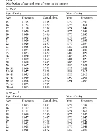
Table 1 indicates that for close to half of male UI claimants (slightly less for women), the year of entry is simply the year in which the T4 file starts, that is 1972. For most of these workers, the year of entry is really a year of entry in the sample as opposed to a year of entry in the work force. For the rest of the sample of claimants, what we call the ‘year of entry’ may either be a true year of entry in the work force or the year of ‘re-entry’ for people who earned some T4 income before 1972 but no T4 income in 1972. Table 1 nevertheless indicates that the age of entry of half of the claimants (age at which T4 income is first recorded) is 20 or less. This suggests that most of the 50.7% of men and 48.6% of women whose year of entry is 1973 or later are not re-entrants in the work force.
Why is it so important to know when a claimant first ‘entered the work force’? The answer is that if we want to find out how previous use of the system affects how long it takes before the person receives UI again, we need to know how long it took before the person used UI for the first time. Since different people join the work force at different times, we need to have some idea of when the person entered the workforce to compute the duration before the first UI spell. Our measure of entry is imperfect since some students earn T4 income during summer
10
jobs even if they have not made a ‘permanent’ transition to the work force. We nevertheless feel this is the best we can do with the available data. We discuss these issues again in Section 4.
We also use information from the T4 Supplementary File to compute a coarse measure of eligibility to UI. We classify as ‘eligible for UI in year t’ individuals who have received some labor income in year t or t21, since people who have not worked at any time during year t and year t21 can never qualify for a new UI benefit period starting in year t. This UI eligibility variable can be used to correct for potential estimation biases likely to arise when people exit the workforce temporarily or permanently because of early retirement, illness, etc.
10
Table 1
Distribution of age and year of entry in the sample a
A. Men
Age of entry Year of entry
Age Frequency Cumul. freq. Year Frequency Cumul. freq.
15 0.105 0.105 1972 0.493 0.493
16 0.124 0.229 1973 0.061 0.553
17 0.110 0.339 1974 0.049 0.602
18 0.079 0.418 1975 0.038 0.640
19 0.049 0.466 1976 0.035 0.675
20 0.035 0.501 1977 0.034 0.709
21 0.029 0.531 1978 0.033 0.742
22 0.026 0.557 1979 0.034 0.776
23 0.025 0.582 1980 0.031 0.807
24 0.024 0.606 1981 0.030 0.837
25 0.023 0.629 1982 0.020 0.857
26 0.020 0.649 1983 0.022 0.879
27 0.019 0.668 1984 0.023 0.902
28 0.018 0.685 1985 0.023 0.925
29 0.017 0.702 1986 0.021 0.946
30–34 0.069 0.771 1987 0.021 0.967
35–39 0.057 0.828 1988 0.013 0.981
40–44 0.055 0.883 1989 0.010 0.991
45–49 0.049 0.932 1990 0.006 0.996
50–54 0.038 0.970 1991 0.004 1.000
55–59 0.025 0.995
60–64 0.005 1.000
b B. Women
Age of entry Year of entry
Age Frequency Cumul. freq. Year Frequency Cumul. freq.
15 0.083 0.083 1972 0.384 0.384
16 0.107 0.191 1973 0.079 0.463
17 0.111 0.301 1974 0.066 0.529
18 0.089 0.390 1975 0.053 0.582
19 0.057 0.447 1976 0.047 0.628
20 0.039 0.486 1977 0.042 0.670
21 0.032 0.519 1978 0.041 0.712
22 0.028 0.546 1979 0.041 0.753
23 0.025 0.572 1980 0.039 0.792
24 0.024 0.596 1981 0.036 0.828
25 0.023 0.619 1982 0.024 0.852
26 0.020 0.639 1983 0.025 0.877
27 0.019 0.658 1984 0.026 0.903
28 0.018 0.675 1985 0.024 0.927
29 0.017 0.692 1986 0.021 0.948
30–34 0.078 0.770 1987 0.019 0.967
35–39 0.069 0.839 1988 0.014 0.981
40–44 0.059 0.898 1989 0.010 0.991
45–49 0.048 0.946 1990 0.006 0.997
50–54 0.033 0.979 1991 0.003 1.000
55–59 0.018 0.997
60–64 0.003 1.000
a
Note: Based on a sample of 618,911 men aged 15 to 65. A person ‘‘enters’’ the sample the first time he receives T4 income between 1972 and 1991.
b
Once the year of entry has been identified in the T4 File, this information is merged to the information about demographic characteristics and UI spells from the Status Vector File. The two files are combined into a yearly panel data file. There is one observation per person in the panel for each year (from the year of entry to 1992). Note that we do not keep an observation in the sample when the person is under 15 or over 65 years old. We also exclude people born before 1912 or after 1972. The resulting sample contains 10 253 535 observations for 618 911 men who have started a UI spell at least once in the years 1972–1992. The comparable sample of women contains 8 074 326 observations for 494 697 women.
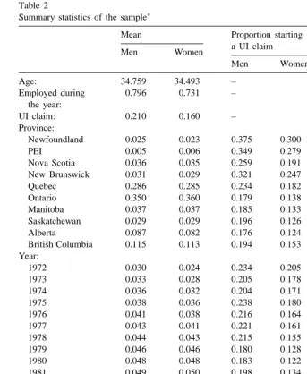
A few statistics on the composition of the samples are reported in Table 2. The average age in the sample is slightly under 35. The regional composition of the sample more or less reflects the relative weight of each province in the national population. Note however, that Quebec and especially the Maritimes are over-represented since a larger fraction of the work force has received UI at least once in these provinces than in provinces west of Quebec.
The table also shows that men in the sample received at least some T4 income in four years out of five and started a UI spell in one year out of five. These proportions are slightly smaller for women. The probability of starting a UI spell is disaggregated by provinces and by year in the second column of Table 2. Once again, there are important East–West differences as people in Quebec and the Maritimes are more likely to start a UI spell than people in other provinces. Not surprisingly, the probability of starting a spell of UI is also counter-cyclical.
4. Difference-in-differences estimates
The descriptive statistics reported in Table 2 do not exploit the longitudinal aspect of the data, nor do they give any indication on how, for example, the past history of UI recipiency is related with the current probability of starting a UI spell. In what follows, we present some descriptive statistics that highlight the dynamic aspects of UI recipiency.
One advantage of working with a large data set like ours is that it is easy to control for observed characteristics by dividing the sample in homogeneous groups of people and doing the analysis separately for each group. In what follows we select three cohort of men and three cohorts of women men born in 1931, 1941 and 1951, respectively. The three particular birth years are selected so that people are old enough to be in the workforce in 1972 and young enough to be in the
11
workforce in 1992.
If learning effects are important, a given experience with the UI system should
11
Table 2
Nova Scotia 0.036 0.035 0.259 0.191
New Brunswick 0.031 0.029 0.321 0.247
Quebec 0.286 0.285 0.234 0.182
Ontario 0.350 0.360 0.179 0.138
Manitoba 0.037 0.037 0.185 0.133
Saskatchewan 0.029 0.029 0.196 0.126
Alberta 0.087 0.082 0.176 0.124
British Columbia 0.115 0.113 0.194 0.153 Year:
have a larger impact on the future probability of receiving UI for people who have no previous experience with the UI system than for people who have some previous experience. One simple measure of the magnitude of learning effects is obtained by comparing the evolution in the probability of UI recipiency of one group of workers that has no previous UI experience with an otherwise compar-able group of workers that has some previous experience.
More concretely, consider a fixed cohort of workers at the beginning of the 1981–1983 recession. Some of these workers have received UI in the past while some others have not. Focusing on the 1981–1983 period is an interesting ‘natural experiment’ since it ‘exposed’ many workers to unemployment and UI recipiency for the first time in their life. If learning is important, the post-recession (e.g. 1984–1986) probability of receiving UI should be higher than the probability that would have prevailed if they had never been exposed to UI. Although this hypothetical probability cannot be directly observed, a control group of workers that were exposed to UI before the recession can be used to calculate the change in the probability of receiving UI between the recession (1981–1983) and the post-recession period (1984–1986) that would have prevailed in the absence of learning effects. Since these workers have already been exposed to the system, a new exposure during the recession should not have any additional effect on the future probability of receiving UI. The change in probability for workers that have been exposed before is thus net of learning effects.
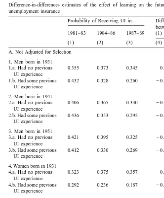
This suggests a simple difference-in-differences estimator of the effect of learning on the probability of using UI. Panel A of Table 3 reports separate difference-in-differences estimates of the effect of learning for the cohorts of men and women born in 1931, 1941 and 1951. Columns 1–3 indicate the probability of receiving UI at least once during the periods 1981–1983, 1984–1986 and 1987– 1989, respectively. These probabilities are simple empirical frequencies for all individuals of the relevant cohorts in the administrative data. While this probability decreases sharply in the post-recession years for workers who had been exposed to UI before the 1981–1983 recession (rows 1b, 2b and 3b), it remains relatively stable, at least for the 1984–1986 period, for workers who had never received UI before the recession. Relatively speaking, a first exposure to UI during the recession increases the probability of receiving UI in the future. These results suggest that part of the upward trend in the use of UI is due to the fact that exposure to the system permanently increases the probability of future use.
Table 3
Difference-in-differences estimates of the effect of learning on the future probability of receiving unemployment insurance
Probability of Receiving UI in: Difference
Difference-between
in-1981–83 1984–86 1987–89 (1) and (2) Differences
(1) (2) (3) (4) (5)
A. Not Adjusted for Selection 1. Men born in 1931
1.a. Had no previous 0.355 0.373 0.345 0.019
UI experience 0.123
1.b. Had some previous 0.432 0.328 0.260 20.104 UI experience
2. Men born in 1941
2.a. Had no previous 0.406 0.365 0.330 20.041
UI experience 0.042
2.b. Had some previous 0.436 0.353 0.295 20.083 UI experience
3. Men born in 1951
3.a. Had no previous 0.421 0.395 0.325 20.026
UI experience 0.056
3.b. Had some previous 0.412 0.330 0.269 20.082 UI experience
4. Women born in 1931
4.a. Had no previous 0.323 0.375 0.357 0.052
UI experience 0.108
4.b. Had some previous 0.292 0.236 0.187 20.056 UI experience
5. Women born in 1941
5.a. Had no previous 0.324 0.379 0.382 0.055
UI experience 0.088
5.b. Had some previous 0.320 0.287 0.247 20.033 UI experience
6. Men born in 1951
6.a. Had no previous 0.300 0.375 0.390 0.075
UI experience 0.089
6.b. Had some previous 0.259 0.245 0.236 20.014 UI experience
number of men born in 1931 included in our data set represent about a half of the
12
total population of men born in 1931 enumerated in the 1981 Canadian Census. We can thus recompute the probabilities of receiving UI for individuals with no
12
Table 3. Continued
Probability of Receiving UI in: Difference
Difference-between
in-1981–83 1984–86 1987–89 (1) and (2) Differences
(1) (2) (3) (4) (5)
B. Adjusted for selection 1. Men born in 1931
1.a. Had no previous 0.104 0.109 0.101 0.006
UI experience 0.109
1.b. Had some previous 0.432 0.328 0.260 20.104 UI experience
2. Men born in 1941
2.a. Had no previous 0.117 0.105 0.095 20.012
UI experience 0.071
2.b. Had some previous 0.436 0.353 0.295 20.083 UI experience
3. Men born in 1951
3.a. Had no previous 0.168 0.158 0.130 20.010
UI experience 0.072
3.b. Had some previous 0.412 0.330 0.269 20.082 UI experience
4. Women born in 1931
4.a. Had no previous 0.094 0.094 0.086 0.000
UI experience 0.104
4.b. Had some previous 0.432 0.328 0.260 20.104 UI experience
5. Women born in 1941
5.a. Had no previous 0.101 0.112 0.110 0.010
UI experience 0.093
5.b. Had some previous 0.436 0.353 0.295 20.083 UI experience
6. Men born in 1951
6.a. Had no previous 0.121 0.146 0.146 0.025
UI experience 0.108
6.b. Had some previous 0.412 0.330 0.269 20.082 UI experience
5. Estimation by random effect probit
In order to look more formally at the dynamics of UI recipiency, consider the following model for the probability that individual i starts a spell of UI in period t:
9 9
Pr(Uit51uUit21, x , L )it it 5F(a 1 d 1 gi t Uit211xitb 1 u0Lit1(xit 1u )L )it
(3)
where i51, . . . ,N, t51, . . . ,T, F(.) is a cumulative distribution function. In this paper, we simply assume that F(.) is a unit normal. The cumulative distribution function F(.) is increasing in its arguments. An increase in arguments such asai or
9
xitb will thus increase the probability that individual i starts a spell of UI in period
t. The arguments in the function F(.) are listed below:
• U , dummy variable equal to one if individual i starts a UI spell during year t;it
• ai, time-invariant random effect;
• dt, aggregate time effect;
• x , vector of covariates including the age of person i, the parameters of the UIit
system in individual i’s region at time t and industry dummies;
• L , a variable indicating whether or not individual i has ‘learned’ how to useit
the UI system at time t. In the simplest version of the learning model, this variable is one if the individual has received UI in the past, and zero otherwise.
In what follows, we refer to L as a learning variable although, more generally,it
it can simply be viewed as a variable indicating whether the person has ever collected UI in the past. The parameter u0 relates the learning variable to the probability of receiving UI, while the vector of parameters u1 indicates whether variables in the vector xit (such as the replacement rate of UI) have a different impact on UI recipiency for people who have learned than for people who have not learned. In other words, u1 captures possible interactions between learning effects and variables such as the parameters of the UI system.
To understand why learning effects can be interpreted as ‘hysteresis’ effects in the use of UI, consider the simple case in whichu1 is equal to zero. From the definition of the learning variable L , it is clear that receiving UI for the first-timeit
switches the learning variable L from 0 to 1 and thus permanently increases theit
probability of receiving UI, provided that u0 is positive. This basic property of learning effects remains whenu1 is different from zero except that the size of the ‘hysteresis’ effect then depends on the value of variables such as replacement and subsidy rates of the UI system.
One difficulty in isolating the importance of learning effects is that many other factors may explain why the history of UI recipiency of a given person i, (U , . . . ,Ui 1 it21), may help predict whether the person will receive UI in period t.
9
standard statistical model for a binary variable with panel data (see Heckman, 1978; Chamberlain, 1980; Heckman, 1981b). In such models, there are two reasons why the history of UI recipiency of a given person i, (U , . . . ,Ui 1 it21), may help predict whether the person will receive UI in period t. First, certain individuals may be more likely to be unemployed and to receive UI because they are less-skilled and / or they have a high marginal valuation of leisure. These factors are summarized by the random person effectai. Since this random effect is by definition fixed for a given person i over time, it increases the probability that the person will receive UI in any time period. As a result, previous use of UI will be strongly correlated with present use of UI since some people are always likely to receive UI (high ai), while some others are not (low ai). This could give the misleading impression that previous use of UI is a cause of the present use of UI. This is called the problem of unobserved heterogeneity.
The history of UI recipiency of a given person i may also help predict whether the person will receive UI in period t because of the presence of the lagged dependent variable Uit21 in Eq. (3). Note that in the estimation we consider models that include further lags of U . We call this particular form of stateit
dependence an adjustment lag. It is natural to expect an adjustment lag in the data for a variety of reasons. For instance, it is well known that the rate of job separation is higher in the first year on a job than in subsequent years (see Farber, 1994). In other words, a job separation is more likely to occur at time t if there was also a separation at time t21 than otherwise. Since UI recipiency is positively correlated with job separations, a UI spell is more likely to be observed in year t if Uit2151 than if Uit2150. Alternatively, workers who have lost some specific human capital because of permanent job displacement may be more likely to be unemployed than if they still had that specific human capital. A UI spell due to permanent job displacement may thus increase the future probability of receiving UI. The key difference between an adjustment lag and learning is that the adjustment lag only temporarily affects the probability of receiving UI, while
13
learning effects are permanent.
Clearly, the fact that the history of UI recipiency (U , . . . ,Ui 1 it21) may help predict whether the person will receive UI in period t is not a proof of the existence of learning effects. The econometric challenge consists of isolating learning effects from the presence of unobserved heterogeneity and adjustment lags. We discuss the econometric strategy in detail below.
One final remark is that the variable L is only a crude measure of learning.it
13
People may also learn how to use the UI system through friends and family. This yields the interesting prediction that the relative role of past UI experience in learning how to use the system should be less important in regions and / or industries in which the use of UI is widespread. One testable implication of this learning model is that the learning coefficient should be lower in high-UI regions such as the Maritimes or Quebec than in low-UI regions such as Ontario or Alberta.
We may also be understating the importance of learning by focusing on learning by individuals only. Since UI is not experience rated in Canada, firms have an incentive to learn along with the worker what is the best way to use the UI system to subsidize part-year work. If this effect is occurring across all firms over time, then the year effects we include in all specifications will absorb learning effects by firms and understate the importance of learning in the whole labor market.
5.1. Estimation methods
Under the assumption that F(.) is a unit normal, the probability that individual i will start a spell of UI in period t can be rewritten as:
9
Prob(Uit51uUit21, L , x ,it it ai)5F(a 1 d 1i t zitv) (4) where:
9 9 9
zitv 5 gUit211xitb 1 u0Lit1(xit 1u )Lit (5) The probability of observing a sequence (U , . . . ,U ) of UI spells is thus equali 1 iT
to:
T
9 Uit 9 ( 12U )it
P
F(a 1 d 1i t zitv) (12F(a 1 d 1i t zitv)) (6)t51
This probability is the essential building block of the likelihood function to be maximized. There are two important issues, however, that need to be addressed before the model can be estimated. First, the probability in Eq. (6) is conditional on a particular value of the random effect ai. Since the random effect is not observed, we need to integrate over its distribution to obtain an unconditional probability of observing the sequence (U , . . . ,U ):i 1 iT
T
9 Uit 9 ( 12U )it
EP
F(a 1 d 1i t zitv) (12F(a 1 d 1i t zitv)) d G(ai) (7)t51
N T
9 Uit 9 ( 12U )it
O
logS
EP
F(a 1 d 1i t zitv) (12F(a 1 d 1i t zitv)) dG(ai)D
(8)t51
i51
Since we have already assumed that the cumulative distribution function F(.) is normal, it seems natural to follow authors like Heckman (1981a) and assume that
G(.) is also normal. In general, evaluating the log-likelihood function (8) requires
some numerical integration, which is computationally burdensome in a large panel data set like the one used here. We thus follow the initial suggestion of Lerman and Manski (1981) of randomly drawing values of ai to evaluate the likelihood
14
function.
To see the basic idea of the simulated maximum likelihood (SML) method, first rewrite the random effect ai as a 5 a 1 si au , where u is a standard normali i
random variable andsais the standard deviation ofai. The log-likelihood function
1 K
We will refer to the estimates obtained by maximizing Eq. (9) as SML
15
estimates. We use K520 in the empirical analysis presented below.
The second important estimation issue arises because of the nature of the administrative files that we use to construct the data set. Since the Status Vector File only contains information on workers who file a UI claim at least once, we have no demographic information on workers who never filed a claim. We thus have to correct for the potential sample selection bias that could result from the way the final sample is constructed.
We correct for sample selection by including some people who never received
16
UI in the sample. Although this cannot be done directly because of the limitations of the administrative data files, some external data sources can be used
14
See also Gourieroux and Monfort (1993) for a recent survey of simulation-based estimation methods.
15
Although SML estimates are only consistent when the number of draws K goes to infinity (Lerman and Manski, 1981; Gourieroux and Monfort, 1993), we noticed in several empirical experiments that there were only small differences between the estimates obtained with 5, 10, 20 or 100 random draws (results from these experiments are available on request).We are thus conservative in using a K as large as 20.
16
to estimate the fraction of people who never received UI. We compute the fraction of individuals who never received UI by combining information from the administrative data with population counts by detailed age groups from the 1981
17
Canadian Census. We then use these estimated fractions to generate a random sample of non-UI recipients who look exactly like UI recipients except that we set their U ’s to zero in all periods. We then maximize the log-likelihood function Eq.it
(9) over a sample composed of the subsample of UI recipients who earned some wage income in 1980 and the ‘artificial’ subsample of non-UI recipients who also earned some wage income in 1980.
A further advantage of the SML method is that it is straightforward to incorporate heterogeneity in other parameters than the intercepta. It seems natural to introduce heterogeneity in the learning parameteru0since a first experience with UI may have different effects on different workers. To introduce heterogeneity in the learning parameter, let:
u 5 u 1 sv
0i 0 u i
wherev is a standard normal variable ands is the standard deviation ofu . The
i u 0i
log-likelihood function can now be approximated by randomly drawing K values
1 K 1 K
Note that u and v will be positively correlated if the learning effect and the
i i
probability of a first experience with UI are both larger for some workers than others. We allow for a possible correlation between heterogeneity in the learning
18
effect and the intercept in the estimation.
Though our model is a random effect model, it is important to point out that it explicitly takes into account the correlation between the person effectai and the explanatory variables related to previous use of UI (Uit21 and L ) since we areit
jointly modeling the probability of receiving UI in all sample years.
5.2. Results
Given the numerical burden associated with maximizing the log-likelihood function, we only perform the estimation over a randomly selected subsample. In order to obtain estimates precise enough for several demographic groups in each
17
See Lemieux and MacLeod (1998) for details. 18
province, we randomly select a 1-in-5 sample for Newfoundland, Nova Scotia, New Brunswick, and Saskatchewan, a 1-in-6 sample for Manitoba, a 1-in-8 sample for Alberta, a 1-in-20 sample for British Columbia, and a 1-in-50 sample for Quebec and Ontario. Prince Edward Island, Yukon and Northwest Territories are excluded from the estimation since these regions cannot be identified separately in the public use release of the 1981 Census micro data.
For both men and women in each province, we further divide the sample in three subsamples based on their year of birth. The first demographic subsample includes individuals born before 1946 who were all old enough to be in the labor force in 1972. The second sample is a sample of ‘baby-boomers’ born from 1946 to 1955, while the third sample of individuals born after 1955 were unlikely to have entered the workforce in 1972. We also limit our analysis to observations that satisfy the ‘eligibility’ rule of having received some T4 income during the current or the previous year. We have also estimated our models without this selection rule and found very similar results.
We first estimate separate models for each of the six demographic groups (two genders and three cohorts) in each province. In each of the 54 random effect probit models, we include the learning variable, the first four lags of the dependent variable (Uit21 to Uit24), age and age squared, and a full set of year and industry dummies. We decided to include four lags of the dependent variable after observing that the estimated effect of further lags was rarely statistically different from zero. The industry dummies are included to ensure that what we call a learning effect is not simply the result of a loss in human capital due to job
19
displacement from an industry to another. Including industry dummies may, however, understate the importance of learning if workers who have just learned about the benefits of the UI program move to an industry where it is easier to work part-year.
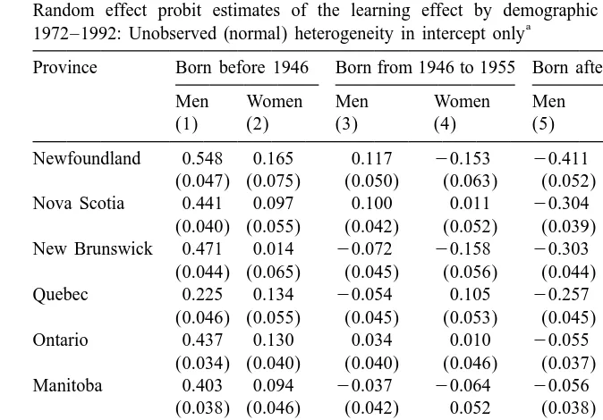
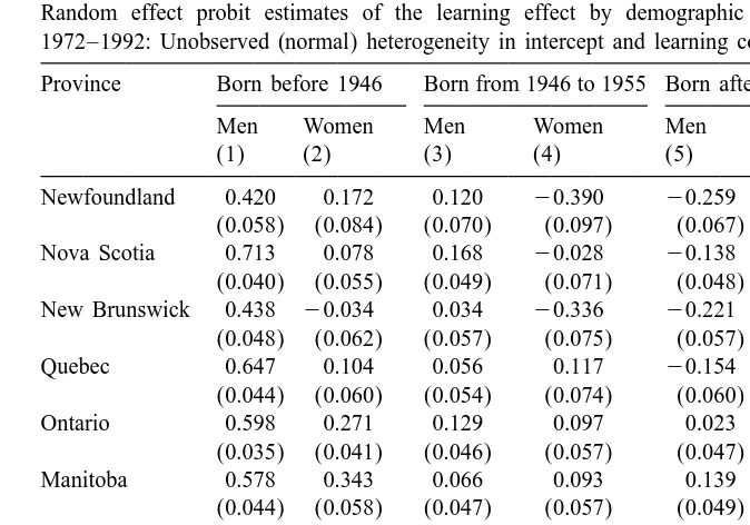
Table 4 reports estimates from models in which unobserved heterogeneity is only included in the intercept. Unobserved heterogeneity is introduced in both the intercept and the learning coefficient in Table 5. We do not include any interactions between the learning variable and other variables in these simple models. The parameteru1 is thus implicitly set to zero.
The estimates of the learning parameteru0 reported in Table 4 are on average positive, but some interesting patterns seem to emerge. First, learning effects tend to be large and positive for men born before 1946 but much smaller and often
19
Table 4
Random effect probit estimates of the learning effect by demographic group and by province, a
1972–1992: Unobserved (normal) heterogeneity in intercept only
Province Born before 1946 Born from 1946 to 1955 Born after 1955
Men Women Men Women Men Women Average
(1) (2) (3) (4) (5) (6) (7)
Newfoundland 0.548 0.165 0.117 20.153 20.411 20.437 20.028 (0.047) (0.075) (0.050) (0.063) (0.052) (0.056)
Nova Scotia 0.441 0.097 0.100 0.011 20.304 20.252 0.016 (0.040) (0.055) (0.042) (0.052) (0.039) (0.049)
New Brunswick 0.471 0.014 20.072 20.158 20.303 20.289 20.056 (0.044) (0.065) (0.045) (0.056) (0.044) (0.050)
Quebec 0.225 0.134 20.054 0.105 20.257 20.091 0.010 (0.046) (0.055) (0.045) (0.053) (0.045) (0.053)
Ontario 0.437 0.130 0.034 0.010 20.055 0.002 0.093 (0.034) (0.040) (0.040) (0.046) (0.037) (0.046)
Manitoba 0.403 0.094 20.037 20.064 20.056 20.034 0.051 (0.038) (0.046) (0.042) 0.052 (0.038) (0.052)
Saskatchewan 0.512 0.129 0.149 20.064 0.042 0.050 0.136 (0.037) (0.056) (0.047) (0.061) (0.035) (0.047)
Alberta 0.505 0.242 0.409 0.249 0.409 0.355 0.361
(0.044) (0.053) (0.046) (0.057) (0.038) (0.047)
British Columbia 0.464 0.136 0.187 0.208 20.007 20.037 0.158 (0.037) (0.053) (0.045) (0.052) (0.041) (0.051)
Average 0.445 0.127 0.093 0.016 20.105 20.082 0.082 a
Note: Standard errors are in parentheses. All models also include a full set of year effects, four lagged values of the dependent variable, age and its squared, and nine industry dummies. Unobserved heterogeneity is accounted for by including a standard normal component in the intercept and estimating the model using simulated maximum likelihood (20 draws).
20
negative for women and younger men. In addition, learning effects are largest in Ontario, Saskatchewan, Alberta and British Columbia, four provinces in which the use of UI is less pervasive than in the rest of the country.
These two patterns of results are consistent with the role of social vs. individual learning mentioned earlier in the text. The more widespread the use of UI is in a region at a point of time, the less previous experience with UI will affect the propensity to use UI. When ‘everybody else’ uses the system, a first experience with the system will not teach a person anything he or she did not already know through family or friends. The results reported in Table 4 thus support the view that younger cohorts of men and women living in areas where the use of UI is
20
Table 5
Random effect probit estimates of the learning effect by demographic group and by province, a
1972–1992: Unobserved (normal) heterogeneity in intercept and learning coefficient Province Born before 1946 Born from 1946 to 1955 Born after 1955
Men Women Men Women Men Women Average
(1) (2) (3) (4) (5) (6) (7)
Newfoundland 0.420 0.172 0.120 20.390 20.259 20.279 20.036 (0.058) (0.084) (0.070) (0.097) (0.067) (0.075)
Nova Scotia 0.713 0.078 0.168 20.028 20.138 20.235 0.093 (0.040) (0.055) (0.049) (0.071) (0.048) (0.055)
New Brunswick 0.438 20.034 0.034 20.336 20.221 20.309 20.071 (0.048) (0.062) (0.057) (0.075) (0.057) (0.068)
Quebec 0.647 0.104 0.056 0.117 20.154 0.022 0.132 (0.044) (0.060) (0.054) (0.074) (0.060) (0.065)
Ontario 0.598 0.271 0.129 0.097 0.023 0.117 0.206
(0.035) (0.041) (0.046) (0.057) (0.047) (0.046)
Manitoba 0.578 0.343 0.066 0.093 0.139 0.205 0.237 (0.044) (0.058) (0.047) (0.057) (0.049) (0.056)
Saskatchewan 0.591 0.174 0.399 20.009 0.016 0.253 0.237 (0.052) (0.062) (0.051) (0.075) (0.046) (0.058)
Alberta 0.757 0.235 0.786 0.744 0.510 0.499 0.588
(0.057) (0.065) (0.058) (0.086) (0.043) (0.064)
British Columbia 0.720 0.410 0.352 0.440 0.035 0.040 0.333 (0.045) (0.061) (0.053) (0.059) (0.054) (0.067)
Average 0.607 0.195 0.234 0.081 20.005 0.035 0.191 a
Note: Standard errors are in parentheses. All models also include a full set of year effects, four lagged values of the dependent variable, age and its squared, and nine industry dummies. Unobserved heterogeneity is accounted for by including a standard normal component in the intercept and the learning coefficient and estimating the model using simulated maximum likelihood (20 draws).
more widespread already knew how the system worked before receiving UI for the first time. It is hard to see how other theories of occurrence dependence such as models of ‘addiction’ or other sources of ‘vicious circles’ could explain the pattern of results reported in Table 4. For example, if people get addicted to UI in the way they get addicted to cigarette smoking, there is no reason why the effect of first-time use of UI would vary across cohorts and regions. By contrast, the substitutability between individual and social learning provides a simple rationali-zation for the patterns observed in the data.
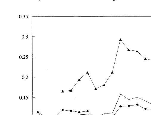
Fig. 3 provides some additional evidence on the role of social vs. individual
21
learning for men. The figure shows the aggregate rate of UI use for the three cohorts of Table 4. The most striking fact is that the youngest cohort enters in the labor market at a much higher rate of UI use than older cohorts. This is consistent with the view that these workers knew about the generosity of the program
21
Fig. 3. UI usage rate by cohort, men.
(through social learning) before they experienced UI for the first time. A second noticeable fact is that the rate of UI use did ratchet up after the 1981–1983 recession for the oldest cohort. It did not ratchet up, however, for the youngest cohort which eventually went back to the pre-recession rate of UI use. This suggests that for individuals in the oldest cohort, a first exposure to UI (through the 1981–1983 recession) had a larger effect on future UI use than for younger cohorts. The evolution of the aggregate UI use rates is, therefore, consistent with the individual vs. social learning interpretation of the results of Table 4.
A more sophisticated interpretation of social learning could also explain why some of the estimated effects in Table 4 are actually negative. If the information gathered through social learning is a bit outdated, it is possible that younger workers who entered the market after the 1971 reform learned socially about the benefits when these were very generous in the 1970s, but then experienced UI for the first time in the 1980s. At that point, they found out that UI was in fact less generous than they first thought which reduced their future propensity to use UI. One testable implication of this hypothesis that we will discuss below is that the learning coefficient should be larger in the 1970s (when people learn UI is more generous than expected) than in the 1980s (when people learn the benefits are no longer as generous as in the 1970s).
We also estimate a pooled version of the model in which we combine the data from the nine provinces for each of the six demographic groups. One advantage of working with a pooled sample is that we can exploit the variation of the parameters of the UI system over regions and time to estimate the effect of these parameters on the propensity to use UI. We combine these UI parameters into a single subsidy rate (see Fig. 1). An increase in the subsidy rate tends to increase the fraction of workers who work part-year and regularly collect UI (Section 2). It should thus have a positive effect on the probability of receiving UI. One interesting hypothesis we can also test in this setting is whether the subsidy rate has a larger effect on people who had some previous experience with the UI system than on people who never had such experience. In terms of Eq. (3), this means that the component of the vector of parameters u1 corresponding to the subsidy rate (one of the elements of x ) should be positive. To ensure that theit
estimated value of this parameter does not simply reflect omitted trends or regional differences in the size of the learning effect, we include (but do not report in the tables) a full set of year and province dummies and interact the learning variable with these dummies.
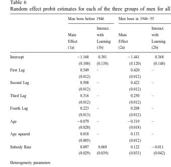
The random effect probit estimates of the pooled models for men are reported in Table 6. The results for women are reported in Table 7. In both cases, we estimate models with unobserved heterogeneity in both the intercept and the learning coefficient. Given the large number of parameters in the estimated models, we only discuss few broad patterns in the results. Two main conclusions emerge from these tables:
1. The subsidy rate always has a positive and significant effect on the probability of receiving UI. These effects are quite small, however, in economic terms. According to the parameter estimates, the impact of a 100% increase in the subsidy rate on the probability of receiving UI is 2–3 percentage points for most of the estimated specifications. The effect of the subsidy rate does not tend to be systematically larger, however, for individuals who have been exposed to UI in the past than for individuals who have not been exposed. 2. The interactions between learning and year effects (not shown in the tables)
show no systematic pattern in the learning effect over time. This is inconsistent with the hypothesis that the learning effect was larger in the 1970s, when workers experiencing UI for the first time found out that the system was more generous than they thought, than in the 1980s when the system was no longer quite as generous. By contrast, the learning effect still tends to be larger for older than for younger cohorts.
Table 6
a Random effect probit estimates for each of the three groups of men for all provinces, 1972–1992
Men born before 1946 Men born in 1946–55 Men born after 1955 Interact. Interact. Interact. Main with Main with Main with Effect Learning Effect Learning Effect Learning (1a) (1b) (2a) (2b) (3a) (3b) Intercept 21.168 0.381 21.441 0.368 21.285 0.068
(0.100) (0.138) (0.120) (0.148) (0.136253) (0.229) First Lag 0.549 – 0.420 – 0.421 –
(0.012) (0.012) (0.012) Second Lag 0.508 – 0.422 – 0.411 –
(0.012) (0.012) (0.011) Third Lag 0.316 – 0.250 – 0.239 –
(0.012) (0.012) (0.011) Fourth Lag 0.223 – 0.208 – 0.145 –
(0.013) (0.012) (0.011) Age 20.079 – 20.319 – 20.491 –
(0.020) (0.018) (0.027) Age squared 0.018 – 0.133 – 20.381 –
(0.005) (0.012) (0.020) Subsidy Rate 0.097 0.069 0.122 20.011 0.120 0.019
(0.029) (0.039) (0.033) (0.042) (0.033) (0.044) Heterogeneity parameters
Variance of 0.4436 0.0456 0.0512 Intercept (0.0311) (0.0099) (0.0073) Variance of 0.0626 0.2024 0.0228 Learning Coeff. (0.0133) (0.0110) (0.0061) Covariance 20.1666 20.0069 0.0321 (0.0169) (0.0050) (0.0047) Observations: 273 600 201 695 169 681
(persons) (16 015) (10 420) (10 547) Log-likelihood: 271 054.8 268 441.8195754 273 401.1
a
Note: The subsidy rate is the UI replacement rate multiplied by the maximum number of weeks of eligibility and divided by the minimum number of weeks to qualify. Unobserved heterogeneity in the intercept and the learning coefficient is modeled as a bivariate standard normal distribution. The model is estimated by simulated maximum likelihood (20 draws). A full set of year and province dummies interacted with the learning variable, as well as nine industry dummies are included in all models.
partly consistent with the idea that individual or social learning about the parameters of the UI system has an impact on employment and unemployment behavior. It could also be consistent, however, with other sources of ‘hysteresis’ coming from the supply side of the market.
Table 7
a Random effect probit estimates for each of the three groups of women for all provinces, 1972–1992
Women born before 1946 Women born in 1946–55 Women born after 1955 Main Interact. Main Interact. Main Interact. effect with effect with effect with (1a) learning (2a) learning (3a) learning
(1b) (2b) (3b)
Intercept 21.217 20.094 21.389 0.142 22.037 0.427 (0.133) (0.187) (0.135) (0.185) (0.184) (0.471) First Lag 0.668 – 0.565 – 0.457 –
(0.016) (0.016) (0.016)
Second Lag 0.588 – 0.502 – 0.441 – (0.017) (0.016) (0.015)
Third Lag 0.339 – 0.338 – 0.276 – (0.017) (0.016) (0.015)
Fourth Lag 0.247 – 0.238 – 0.134 – (0.018) (0.017) (0.016)
Age 20.126 – 20.058 – 20.406 – (0.027) (0.021) (0.032)
Age squared 0.018 – 0.011 – 20.370 – (0.007) (0.014) (0.026)
Subsidy Rate 0.100 0.144 0.181 20.079 0.281 20.162 (0.037) (0.053) (0.038) (0.052) (0.035) (0.054) Heterogeneity parameters
Variance of 0.4206 0.0916 0.0943 Intercept (0.0369) (0.0145) (0.0139) Variance of 0.1450 0.0021 0.0011
Learning Coeff. (0.0246) (0.0020) (0.0015) Covariance 20.2309 0.0027 0.0050
(0.0221) (0.0073) (0.0070) Observations: 173 248 141 428 138 012 (persons) (10 774) (7751) (9058) Log-likelihood: 242 926.2 241 914.8 246 000.2
a
Note: The subsidy rate is the UI replacement rate multiplied by the maximum number of weeks of eligibity and divided by the minimum number of weeks to qualify. Unobserved heterogeneity in the intercept and the learning coefficient is modeled as a bivariate standard normal distribution. The model is estimated by simulated maximum likelihood (20 draws). A full set of year and province dummies interacted with the learning variable, as well as nine industry dummies are included in all models.
22
fixed effects. Interestingly, McCall (1999) obtained similar results for the United States using a linear probability model with fixed effects. This suggests that our results do not simply reflect some spurious features of the Canadian labor market.
22
6. Summary of the findings: how big are the learning effects?
Both the difference-in-differences approach and the random effect probit model suggest that learning plays a role in the probability of receiving UI. We first present some simple ‘back-of-the-envelope’ calculations that suggest that learning effects may be large enough to explain a substantial fraction of the 2–2.5 percentage point gap in unemployment rates between Canada and the United States that emerged in the early 1980s.
To see this, first notice that both the difference-in-differences and the random effect probit estimates indicate that a first exposure to UI increases, on average, the future probability of receiving UI by 3–4 percentage points a year. This is easily seen for the difference-in-differences models for which a first exposure increases the probability of future use by around 10 percentage points over a 3-year period
23
(Table 3), or at least 3–4 percentage points a year.
In the case of the random effect probit model, the effect of learning on the probability of receiving UI depends on workers’ type (unobserved heterogeneity) as well as on the size of the learning parameter. Consider a learning parameter of 0.2 (average of the parameters in Table 5) and a variance of unobserved heterogeneity of 0.27 (average estimated value). In this case, the effect of learning on the future probability of receiving UI varies from 5 percentage points for less-skilled workers (5th percentile of the distribution of unobserved hetero-geneity) to 1% for highly-skilled workers (95th percentile of the distribution of unobserved heterogeneity). The average effect is around 3 percentage points,
24
which is comparable to the difference-in-differences estimates.
Since over 50% of individuals in the sample period eventually receive UI at least once, learning effects can potentially explain a 1.5–2 percentage points
25
increase in the probability of receiving UI. . If there was a one-to-one mapping between UI and unemployment, as Fig. 2 suggests, this would mean that learning effects account for a substantial fraction of Canada–US unemployment rate gap
26
that emerged in the 1980s.
23
Since many workers receive UI more than once over a 3-year period, the yearly probability exceeds a third of the probability over a 3-year period.
24
Using a variance of unobserved heterogeneity smaller than 0.27 yields the same average effect of learning. It simply reduces the effect for less-skilled workers and increases the effect for highly-skilled workers, leaving the average effect virtually unchanged.
25
The 50% figure is obtained by comparing the number of people in the sample to total population counts in the 1981 Canadian Census.
26
Fig. 4. Simulated impact of learning on UI usage rate, men.
In Fig. 4, we present a more detailed simulation of the impact of learning on the
27
rate of UI use for men. This simulation consists of setting the learning coefficient (main effect plus interactions) to zero in the model presented in Table 6, and then simulating the UI usage rate that would prevail in the absence of learning effects. The impact of learning on the UI usage rate is the difference between the actual UI usage rate and the simulated UI usage rate. The figure shows that until the recession of 1981–1983, which was the worst recession in Canada since the Great Depression, learning had little impact on the UI usage rate. The impact of learning was to ratchet up the UI usage in the years following the recession. This is consistent with the view that a first exposure to UI during the recession had a permanent effect on the future propensity to collect UI.
The results reported in Fig. 4 suggest that learning is a source of supply side hysteresis in the usage rate of UI. That is, a negative labor market shock like the recession of 1981–1983 can have a permanent effect on the usage rate of UI as many workers learn for the first time about the benefits of UI through this bout of unemployment. To the extent that UI recipiency is closely connected with being unemployed, our results also suggest that learning about UI may also be a source of hysteresis in the unemployment rate.
27
7. Concluding remarks
We find some mixed evidence that first-time use of the unemployment insurance system in Canada increases the probability of future use. As workers are exposed to UI for the first time for a variety of reasons, they learn about the functioning of the system and adjust their behavior accordingly.
This behavior is consistent with individuals responding to the incentives provided by the system. The fact that experience is required for a change in behavior is consistent with laboratory studies of learning. It also suggests that studies based on cross-section estimates of supply responses underestimate the long-term impact of the disincentive effects of social welfare programs.
In Canada’s case, the increased divergence of the Canadian and American unemployment rates has long been a source of concern. The study of Card and Riddell (1993) is unable to identify the source of the difference based upon a standard supply and demand analysis. The lagged adjustment effects identified in this study may provide a coherent explanation for this effect. Given the size of the 1971 changes to the UI system, even as benefits decreased in the subsequent 20 years, workers unfamiliar with the system may still modify their behavior after a spell of unemployment several years after the change because they had never considered part-year work as an option. The results reported in Fig. 4 are consistent with this explanation.
If subsequent research supports this conjecture, this has potentially important implications for the design of social welfare programs. Specifically it would imply that the feedback between a policy change, and its ultimate impact on the economy may be very slow, and hence it suggests that it may be very costly to learn about and correct policy errors. Moreover, once individuals have adjusted their behavior to the system, one is likely to face a similar lagged adjustment in the reverse direction as individuals take time to learn and respond to the new parameters. Canada has recently tightened significantly its UI rules. It will be interesting to see how the Canada–US unemployment rate gap responds as a consequence.
Secondly, this highlights the importance of coverage in determining the impact of changes in a program. Rule changes that affect current recipients can be expected to have an immediate impact because the individuals experience the rule change. However, for program rule changes that involve an increase in the target population, our results suggest that it may take some time before the new
28
individuals at risk respond fully to the new incentives. In summary these results suggest that great care must be taken if we are to properly interpret the relationship
28
between changes in incentives at the individual level, and the subsequent impact on the economy as a whole.
Acknowledgements
We would like to thank Janet Currie, Chris Ferrall, Roger Gordon, Christian ´
Gourieroux, Phillip Levine, David Neumark, Anne Routhier, Ging Wong, and two anonymous referees for helpful comments, Ali Bejaoui for research assistance, and the following for financial support: FCAR, SSHRC, HRDC and NSF (Grant No. SBR-9709333).
References
Alchian, A.A., 1950. Uncertainty, evolution and economic theory. Journal of Political Economy 58, 211–221.
Bandura, A., 1986. Social Foundations of Thought and Action. Prentice-Hall, Englewood Cliffs, NJ. Bloom, H., Fink, B., Lui-Gurr, S., Bancroft, W., Tattrie, D., 1997. Implementing the earnings supplement project: A test of a re-employment incentive. Social Research and Demonstration Corporation, Ottawa, Canada.
Card, D., Riddell, W.C., 1993. A comparative analysis of unemployment in the United States and Canada. In: Card, D., Freeeman, R.B. (Eds.), Small Differences that Matter: Labor Markets and Income Maintenance in Canada and the United States. University of Chicago Press, Chicago, pp. 149–189.
Chamberlain, G., 1980. Analysis of covariance with qualitative data. Review of Economic Studies 47, 225–238.
Corak, M., 1993. Unemployment insurance once again: The incidence of repeat participation in the Canadian UI program. Canadian Public Policy 19, 162–176.
Currie, J., 1995. Welfare and the well-being of children. Fundamentals of Pure and Applied Economics, Vol. 59. Harwood Academic Publishers, Chur, Switzerland.
Farber, H.S., 1994. The analysis of interfirm worker mobility. Journal of Labor Economics 12, 554–593.
Gourieroux, C., Monfort, A., 1993. Simulation-based inference: A survey with special reference to panel data models. Journal of Econometrics 59, 5–34.
Green, D.A., Riddell, W.C., 1993. The economic effect of unemployment insurance in Canada: An empirical analysis of UI disentitlement. Journal of Labor Economics 11, S96–S147.
Ham, J., Rea, S., 1987. Unemployment insurance and male unemployment duration in Canada. Journal of Labor Economics 5, 325–351.
Heckman, J.J., 1978. Simple statistical models for discrete panel data developed and applied to test the hypothesis of true state dependence against the spurious state dependence. Annales de l’INSEE 30, 227–269.
Heckman, J.J., 1981a. Statistical models for discrete panel data. In: Manski, C.F., McFadden, D. (Eds.), Structural Analysis of Discrete Data with Econometric Applications. MIT Press, Cambridge, MA, pp. 114–178.
Manski, C.F., McFadden, D. (Eds.), Structural Analysis of Discrete Data with Economic Applica-tions. MIT Press, Cambridge, MA, pp. 179–195.
Heckman, J.J., Borjas, G., 1980. Does unemployment cause future unemployment? Definitions, questions and answers from a continuous time model of heterogeneity and state dependence. Economica 47, 247–283.
Katz, L.F., Meyer, B.D., 1990. Unemployment insurance, recall expectations, and unemployment outcomes. Quarterly Journal of Economics 105, 973–1002.
Knight, F.H., 1921. Risk, Uncertainty, and Profit. Hart, Schaffner, and Marx, New York.
Layard, R., Nickell, S., Jackman, R., 1991. Unemployment, Macroeconomic Performance and the Labour Market. Oxford University Press, Oxford, UK.
Lerman, S.R., Manski, C.F., 1981. On the use of simulated frequencies to approximate choice probabilities. In: Manski, C.F., McFadden, D. (Eds.), Structural Analysis of Discrete Data with Econometric Applications. MIT Press, Cambridge, MA, pp. 305–319.
Lemieux, T., MacLeod, W.B., 1998. Supply side hysteresis: The case of the Canadian unemployment insurance system. Working Paper No. 6732, National Bureau of Economic Research.
Lindbeck, A., 1995. Welfare state disincentives with endogenous habits and norms. Scandinavian Journal of Economics 97, 477–494.
Marshall, A., 1948. The Principles of Economics. MacMillan, New York.
McCall, B.P., 1999. Repeat use of unemployment insurance. In: Bassi, L.J., Woodbury, S.A. (Eds.). Research in Employment Policies, Vol. 2. JAI Press, Stamford, CT.
Meyer, B., 1990. Unemployment insurance and unemployment spells. Econometrica 58, 757–782. Meyer, B.D., Rosenbaum, D.T., 1996. Repeat use of unemployment insurance. Working Paper No.
5423, National Bureau of Economic Research.
Moffit, R., 1992. Incentive effects of the US welfare system: A review. Journal of Economic Literature 30, 1–61.
Savage, L.J., 1972. The Foundations of Statistics. Dover Publications, New York.
Simon, H.A., 1956. Rational choice and the structure on the environment. Psychological Review 63, 129–138.
Topel, R.H., 1983. On layoffs and unemployment insurance. American Economic Review 73, 541–559. Wickens, C., 1992. Engineering Psychology and Human Performance, 2nd Edition. Harper Collins,
New York.